Data transferred from (GitHub Address ):https://github.com/wesm/pydata-book Friends in need can go by themselves github download 
The time series (time series) Data is an important form of structured data , It can be used in many fields , Including finance 、 economics 、 Ecology 、 neuroscience 、 Physics, etc . Anything observed or measured at multiple time points can form a time series . A lot of time series are fixed frequency , in other words , Data points appear regularly according to some rule ( Like every 15 second 、 Every time 5 minute 、 Once a month ). Time series can also be irregular , There are no fixed time units or offsets between units . The significance of time series data depends on the specific application scenario , There are mainly the following :
This chapter is mainly about 3 Time series . Many techniques can be used to deal with experimental time series , Its index may be an integer or floating point number ( Indicates the time elapsed since the beginning of the experiment ). The simplest and most common time series are indexed with time stamps .
Tips :pandas Also support based on timedeltas The index of , It can effectively represent the experiment or elapsed time . This book does not cover timedelta Index , But you can learn pandas Documents (http://pandas.pydata.org/).
pandas It provides many built-in time series processing tools and data algorithms . therefore , You can efficiently handle very large time series , Slice easily / cutting 、 polymerization 、 On a regular basis / Re sampling of irregular time series, etc . Some tools are especially suitable for financial and economic applications , You can also use them to analyze server log data .
Python The standard library contains information for dates (date) And time (time) The data type of the data , And there are calendar functions . We will mainly use datetime、time as well as calendar modular .datetime.datetime( Or we could just write it as datetime) Is the most used data type :
In [10]: from datetime import datetime
In [11]: now = datetime.now()
In [12]: now
Out[12]: datetime.datetime(2017, 9, 25, 14, 5, 52, 72973)
In [13]: now.year, now.month, now.day
Out[13]: (2017, 9, 25)
datetime Store date and time in milliseconds .timedelta Two datetime Time difference between objects :
In [14]: delta = datetime(2011, 1, 7) - datetime(2008, 6, 24, 8, 15)
In [15]: delta
Out[15]: datetime.timedelta(926, 56700)
In [16]: delta.days
Out[16]: 926
In [17]: delta.seconds
Out[17]: 56700
You can give datetime Object plus ( Or subtract ) One or more timedelta, This creates a new object :
In [18]: from datetime import timedelta
In [19]: start = datetime(2011, 1, 7)
In [20]: start + timedelta(12)
Out[20]: datetime.datetime(2011, 1, 19, 0, 0)
In [21]: start - 2 * timedelta(12)
Out[21]: datetime.datetime(2010, 12, 14, 0, 0)
datetime See table for data types in the module 10-1. Although this chapter mainly talks about pandas Data types and advanced time series processing , But you will definitely be Python Encountered in other places about datetime Data type of .
surface 11-1 datetime Data types in modules
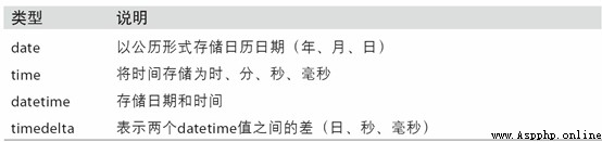
tzinfo The basic type for storing time zone information
utilize str or strftime Method ( Pass in a formatted string ),datetime Objects and pandas Of Timestamp object ( I'll introduce it later ) Can be formatted as a string :
In [22]: stamp = datetime(2011, 1, 3)
In [23]: str(stamp)
Out[23]: '2011-01-03 00:00:00'
In [24]: stamp.strftime('%Y-%m-%d')
Out[24]: '2011-01-03'
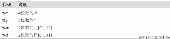
surface 11-2 Lists all formatting codes .
surface 11-2 datetime Format definition ( compatible ISO C89)
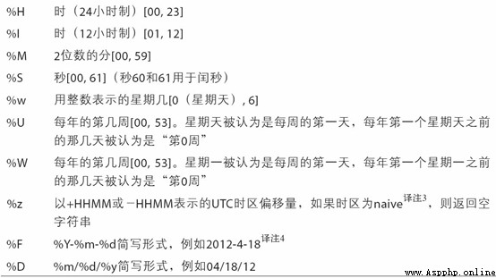
datetime.strptime You can use these formatting encodings to convert a string to a date :
In [25]: value = '2011-01-03'
In [26]: datetime.strptime(value, '%Y-%m-%d')
Out[26]: datetime.datetime(2011, 1, 3, 0, 0)
In [27]: datestrs = ['7/6/2011', '8/6/2011']
In [28]: [datetime.strptime(x, '%m/%d/%Y') for x in datestrs]
Out[28]:
[datetime.datetime(2011, 7, 6, 0, 0),
datetime.datetime(2011, 8, 6, 0, 0)]
datetime.strptime It's the best way to parse dates in a known format . But it's troublesome to write a format definition every time , Especially for some common date formats . In this case , You can use it. dateutil In this third party package parser.parse Method (pandas It's already installed automatically in ):
In [29]: from dateutil.parser import parse
In [30]: parse('2011-01-03')
Out[30]: datetime.datetime(2011, 1, 3, 0, 0)
dateutil You can parse almost all the date representations that humans can understand :
In [31]: parse('Jan 31, 1997 10:45 PM')
Out[31]: datetime.datetime(1997, 1, 31, 22, 45)
In the international format , It is common for the sun to appear before the month , Pass in dayfirst=True To solve this problem :
In [32]: parse('6/12/2011', dayfirst=True)
Out[32]: datetime.datetime(2011, 12, 6, 0, 0)
pandas Usually used to handle group dates , Whether these dates are DataFrame Axis index or column .to_datetime Method can parse many different date representations . For standard date formats ( Such as ISO8601) It's very fast :
In [33]: datestrs = ['2011-07-06 12:00:00', '2011-08-06 00:00:00']
In [34]: pd.to_datetime(datestrs)
Out[34]: DatetimeIndex(['2011-07-06 12:00:00', '2011-08-06 00:00:00'], dtype='dat
etime64[ns]', freq=None)
It can also handle missing values (None、 Empty string, etc ):
In [35]: idx = pd.to_datetime(datestrs + [None])
In [36]: idx
Out[36]: DatetimeIndex(['2011-07-06 12:00:00', '2011-08-06 00:00:00', 'NaT'], dty
pe='datetime64[ns]', freq=None)
In [37]: idx[2]
Out[37]: NaT
In [38]: pd.isnull(idx)
Out[38]: array([False, False, True], dtype=bool)
NaT(Not a Time) yes pandas Time stamp data in null value .
Be careful :dateutil.parser It's a practical but imperfect tool . for instance , It takes strings that are not dates as dates ( such as "42" It will be resolved to 2042 Years of today ).
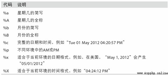
datetime Objects also have some that are specific to the current environment ( Systems located in different countries or languages ) Format options for . for example , The month abbreviations used in the German or French system are different from those used in the English system . surface 11-3 It is summarized .
surface 11-3 Date format specific to the current environment
pandas The most basic type of time series is time stamp ( Usually, the Python String or datatime Objects represent ) For index Series:
In [39]: from datetime import datetime
In [40]: dates = [datetime(2011, 1, 2), datetime(2011, 1, 5),
....: datetime(2011, 1, 7), datetime(2011, 1, 8),
....: datetime(2011, 1, 10), datetime(2011, 1, 12)]
In [41]: ts = pd.Series(np.random.randn(6), index=dates)
In [42]: ts
Out[42]:
2011-01-02 -0.204708
2011-01-05 0.478943
2011-01-07 -0.519439
2011-01-08 -0.555730
2011-01-10 1.965781
2011-01-12 1.393406
dtype: float64
these datetime Objects are actually placed in a DatetimeIndex Medium :
In [43]: ts.index
Out[43]:
DatetimeIndex(['2011-01-02', '2011-01-05', '2011-01-07', '2011-01-08',
'2011-01-10', '2011-01-12'],
dtype='datetime64[ns]', freq=None)
With others Series equally , Arithmetic operations between time series of different indexes are automatically aligned by date :
In [44]: ts + ts[::2]
Out[44]:
2011-01-02 -0.409415
2011-01-05 NaN
2011-01-07 -1.038877
2011-01-08 NaN
2011-01-10 3.931561
2011-01-12 NaN
dtype: float64
ts[::2] Is to take one every two .
pandas use NumPy Of datetime64 Data types store timestamps in nanoseconds :
In [45]: ts.index.dtype
Out[45]: dtype('<M8[ns]')
DatetimeIndex The scalar values in are pandas Of Timestamp object :
In [46]: stamp = ts.index[0]
In [47]: stamp
Out[47]: Timestamp('2011-01-02 00:00:00')
As long as there is a need ,TimeStamp It can be automatically converted to at any time datetime object . Besides , It can also store frequency information ( If any ), And know how to perform time zone conversion and other operations . More on this later .
When you select data based on the tag index , Time series and other pandas.Series It's like :
In [48]: stamp = ts.index[2]
In [49]: ts[stamp]
Out[49]: -0.51943871505673811
There is a more convenient use : Pass in a string that can be interpreted as a date :
In [50]: ts['1/10/2011']
Out[50]: 1.9657805725027142
In [51]: ts['20110110']
Out[51]: 1.9657805725027142
For longer time series , Just incoming “ year ” or “ years ” You can easily select slices of data :
In [52]: longer_ts = pd.Series(np.random.randn(1000),
....: index=pd.date_range('1/1/2000', periods=1000))
In [53]: longer_ts
Out[53]:
2000-01-01 0.092908
2000-01-02 0.281746
2000-01-03 0.769023
2000-01-04 1.246435
2000-01-05 1.007189
2000-01-06 -1.296221
2000-01-07 0.274992
2000-01-08 0.228913
2000-01-09 1.352917
2000-01-10 0.886429
...
2002-09-17 -0.139298
2002-09-18 -1.159926
2002-09-19 0.618965
2002-09-20 1.373890
2002-09-21 -0.983505
2002-09-22 0.930944
2002-09-23 -0.811676
2002-09-24 -1.830156
2002-09-25 -0.138730
2002-09-26 0.334088
Freq: D, Length: 1000, dtype: float64
In [54]: longer_ts['2001']
Out[54]:
2001-01-01 1.599534
2001-01-02 0.474071
2001-01-03 0.151326
2001-01-04 -0.542173
2001-01-05 -0.475496
2001-01-06 0.106403
2001-01-07 -1.308228
2001-01-08 2.173185
2001-01-09 0.564561
2001-01-10 -0.190481
...
2001-12-22 0.000369
2001-12-23 0.900885
2001-12-24 -0.454869
2001-12-25 -0.864547
2001-12-26 1.129120
2001-12-27 0.057874
2001-12-28 -0.433739
2001-12-29 0.092698
2001-12-30 -1.397820
2001-12-31 1.457823
Freq: D, Length: 365, dtype: float64
here , character string “2001” Be interpreted as an adult , And select the time interval according to it . A given month also works :
In [55]: longer_ts['2001-05']
Out[55]:
2001-05-01 -0.622547
2001-05-02 0.936289
2001-05-03 0.750018
2001-05-04 -0.056715
2001-05-05 2.300675
2001-05-06 0.569497
2001-05-07 1.489410
2001-05-08 1.264250
2001-05-09 -0.761837
2001-05-10 -0.331617
...
2001-05-22 0.503699
2001-05-23 -1.387874
2001-05-24 0.204851
2001-05-25 0.603705
2001-05-26 0.545680
2001-05-27 0.235477
2001-05-28 0.111835
2001-05-29 -1.251504
2001-05-30 -2.949343
2001-05-31 0.634634
Freq: D, Length: 31, dtype: float64
datetime Objects can also be sliced :
In [56]: ts[datetime(2011, 1, 7):]
Out[56]:
2011-01-07 -0.519439
2011-01-08 -0.555730
2011-01-10 1.965781
2011-01-12 1.393406
dtype: float64
Because most of the time series data are sorted in chronological order , So you can also slice it with timestamps that don't exist in the time series ( Range query ):
In [57]: ts
Out[57]:
2011-01-02 -0.204708
2011-01-05 0.478943
2011-01-07 -0.519439
2011-01-08 -0.555730
2011-01-10 1.965781
2011-01-12 1.393406
dtype: float64
In [58]: ts['1/6/2011':'1/11/2011']
Out[58]:
2011-01-07 -0.519439
2011-01-08 -0.555730
2011-01-10 1.965781
dtype: float64
Same as before , You can pass in a string date 、datetime or Timestamp. Be careful , What this slice produces is a view of the original time series , Follow NumPy Array slicing is the same .
It means , No data copied , Changes to the slice are reflected in the original data .
Besides , There is also an equivalent instance method that can intercept between two dates TimeSeries:
In [59]: ts.truncate(after='1/9/2011')
Out[59]:
2011-01-02 -0.204708
2011-01-05 0.478943
2011-01-07 -0.519439
2011-01-08 -0.555730
dtype: float64
These operations are right DataFrame It works . for example , Yes DataFrame Index the rows of :
In [60]: dates = pd.date_range('1/1/2000', periods=100, freq='W-WED')
In [61]: long_df = pd.DataFrame(np.random.randn(100, 4),
....: index=dates,
....: columns=['Colorado', 'Texas',
....: 'New York', 'Ohio'])
In [62]: long_df.loc['5-2001']
Out[62]:
Colorado Texas New York Ohio
2001-05-02 -0.006045 0.490094 -0.277186 -0.707213
2001-05-09 -0.560107 2.735527 0.927335 1.513906
2001-05-16 0.538600 1.273768 0.667876 -0.969206
2001-05-23 1.676091 -0.817649 0.050188 1.951312
2001-05-30 3.260383 0.963301 1.201206 -1.852001
In some application scenarios , There may be multiple observation data falling on the same time point . Here is an example :
In [63]: dates = pd.DatetimeIndex(['1/1/2000', '1/2/2000', '1/2/2000',
....: '1/2/2000', '1/3/2000'])
In [64]: dup_ts = pd.Series(np.arange(5), index=dates)
In [65]: dup_ts
Out[65]:
2000-01-01 0
2000-01-02 1
2000-01-02 2
2000-01-02 3
2000-01-03 4
dtype: int64
By checking the index is_unique attribute , We can know if it is the only :
In [66]: dup_ts.index.is_unique
Out[66]: False
Index this time series , Or generate scalar values , Or produce slices , It depends on whether the selected time point is repeated :
In [67]: dup_ts['1/3/2000'] # not duplicated
Out[67]: 4
In [68]: dup_ts['1/2/2000'] # duplicated
Out[68]:
2000-01-02 1
2000-01-02 2
2000-01-02 3
dtype: int64
Suppose you want to aggregate data with non unique timestamps . One way is to use groupby, And pass in level=0:
In [69]: grouped = dup_ts.groupby(level=0)
In [70]: grouped.mean()
Out[70]:
2000-01-01 0
2000-01-02 2
2000-01-03 4
dtype: int64
In [71]: grouped.count()
Out[71]:
2000-01-01 1
2000-01-02 3
2000-01-03 1
dtype: int64
pandas The original time series in are generally considered to be irregular , in other words , They don't have a fixed frequency . For most applications , It doesn't matter . however , It often needs to be analyzed at a relatively fixed frequency , Like every day 、 monthly 、 Every time 15 Minutes, etc ( This will naturally introduce missing values into the time series ). Fortunately, ,pandas There's a whole set of standard time series frequencies and for resampling 、 Frequency inference 、 Tools for generating fixed frequency date ranges . for example , We can convert the previous time series into a time series with a fixed frequency ( everyday ) Time series of , Just call resample that will do :
In [72]: ts
Out[72]:
2011-01-02 -0.204708
2011-01-05 0.478943
2011-01-07 -0.519439
2011-01-08 -0.555730
2011-01-10 1.965781
2011-01-12 1.393406
dtype: float64
In [73]: resampler = ts.resample('D')
character string “D” It means every day .
Frequency conversion ( Or resampling ) It's a big theme , A section will be devoted to the discussion later (11.6 Section ). here , I'll show you how to use the basic frequency and its multiples .
Although I didn't say it clearly when I used it before , But you may have guessed pandas.date_range Can be used to generate a specified length of DatetimeIndex:
In [74]: index = pd.date_range('2012-04-01', '2012-06-01')
In [75]: index
Out[75]:
DatetimeIndex(['2012-04-01', '2012-04-02', '2012-04-03', '2012-04-04',
'2012-04-05', '2012-04-06', '2012-04-07', '2012-04-08',
'2012-04-09', '2012-04-10', '2012-04-11', '2012-04-12',
'2012-04-13', '2012-04-14', '2012-04-15', '2012-04-16',
'2012-04-17', '2012-04-18', '2012-04-19', '2012-04-20',
'2012-04-21', '2012-04-22', '2012-04-23', '2012-04-24',
'2012-04-25', '2012-04-26', '2012-04-27', '2012-04-28',
'2012-04-29', '2012-04-30', '2012-05-01', '2012-05-02',
'2012-05-03', '2012-05-04', '2012-05-05', '2012-05-06',
'2012-05-07', '2012-05-08', '2012-05-09', '2012-05-10',
'2012-05-11', '2012-05-12', '2012-05-13', '2012-05-14',
'2012-05-15', '2012-05-16', '2012-05-17', '2012-05-18',
'2012-05-19', '2012-05-20', '2012-05-21', '2012-05-22',
'2012-05-23', '2012-05-24', '2012-05-25', '2012-05-26',
'2012-05-27', '2012-05-28', '2012-05-29', '2012-05-30',
'2012-05-31', '2012-06-01'],
dtype='datetime64[ns]', freq='D')
By default ,date_range It produces a point in time by day . If only the start or end date is passed in , Then you have to pass in a number that represents a period of time :
In [76]: pd.date_range(start='2012-04-01', periods=20)
Out[76]:
DatetimeIndex(['2012-04-01', '2012-04-02', '2012-04-03', '2012-04-04',
'2012-04-05', '2012-04-06', '2012-04-07', '2012-04-08',
'2012-04-09', '2012-04-10', '2012-04-11', '2012-04-12',
'2012-04-13', '2012-04-14', '2012-04-15', '2012-04-16',
'2012-04-17', '2012-04-18', '2012-04-19', '2012-04-20'],
dtype='datetime64[ns]', freq='D')
In [77]: pd.date_range(end='2012-06-01', periods=20)
Out[77]:
DatetimeIndex(['2012-05-13', '2012-05-14', '2012-05-15', '2012-05-16',
'2012-05-17', '2012-05-18', '2012-05-19', '2012-05-20',
'2012-05-21', '2012-05-22', '2012-05-23', '2012-05-24',
'2012-05-25', '2012-05-26', '2012-05-27','2012-05-28',
'2012-05-29', '2012-05-30', '2012-05-31', '2012-06-01'],
dtype='datetime64[ns]', freq='D')
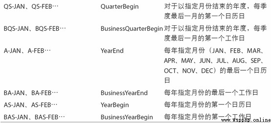
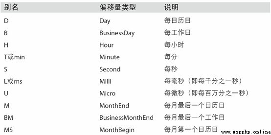
The start and end dates define the strict boundaries of the date index . for example , If you want to generate a date index consisting of the last working day of each month , You can pass in "BM" frequency ( Express business end of month, surface 11-4 It's a list of frequencies ), This will only include time intervals ( Or just on the border ) Dates that meet the frequency requirements :
In [78]: pd.date_range('2000-01-01', '2000-12-01', freq='BM')
Out[78]:
DatetimeIndex(['2000-01-31', '2000-02-29', '2000-03-31', '2000-04-28',
'2000-05-31', '2000-06-30', '2000-07-31', '2000-08-31',
'2000-09-29', '2000-10-31', '2000-11-30'],
dtype='datetime64[ns]', freq='BM')
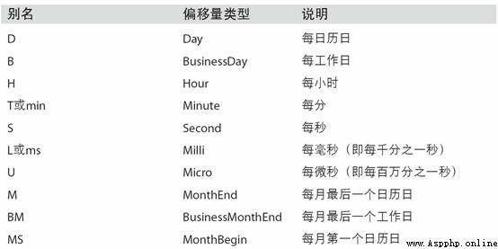
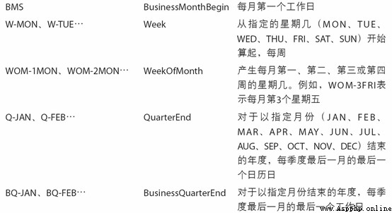
surface 11-4 Basic time series frequency ( Incomplete )
date_range By default, the time information of the start and end timestamps will be retained ( If any ):
In [79]: pd.date_range('2012-05-02 12:56:31', periods=5)
Out[79]:
DatetimeIndex(['2012-05-02 12:56:31', '2012-05-03 12:56:31',
'2012-05-04 12:56:31', '2012-05-05 12:56:31',
'2012-05-06 12:56:31'],
dtype='datetime64[ns]', freq='D')
Sometimes , Although the start and end dates have time information , But you want to produce a set of standardized (normalize) Time stamp to midnight .normalize Option to achieve this function :
In [80]: pd.date_range('2012-05-02 12:56:31', periods=5, normalize=True)
Out[80]:
DatetimeIndex(['2012-05-02', '2012-05-03', '2012-05-04', '2012-05-05',
'2012-05-06'],
dtype='datetime64[ns]', freq='D')
pandas The frequency in is determined by a fundamental frequency (base frequency) And a multiplier . The base frequency is usually represented by a string alias , such as "M" Means every month ,"H" Every hour . For each fundamental frequency , There's a date offset called (date offset) Corresponding to the object of . for example , The frequency in hours can be calculated by Hour Class represents :
In [81]: from pandas.tseries.offsets import Hour, Minute
In [82]: hour = Hour()
In [83]: hour
Out[83]: <Hour>
Pass in an integer to define the multiple of the offset :
In [84]: four_hours = Hour(4)
In [85]: four_hours
Out[85]: <4 * Hours>
Generally speaking , There is no need to explicitly create such an object , Just use something like "H" or "4H" Such a string alias is sufficient . A multiple can be created by placing an integer in front of the base frequency :
In [86]: pd.date_range('2000-01-01', '2000-01-03 23:59', freq='4h')
Out[86]:
DatetimeIndex(['2000-01-01 00:00:00', '2000-01-01 04:00:00',
'2000-01-01 08:00:00', '2000-01-01 12:00:00',
'2000-01-01 16:00:00', '2000-01-01 20:00:00',
'2000-01-02 00:00:00', '2000-01-02 04:00:00',
'2000-01-02 08:00:00', '2000-01-02 12:00:00',
'2000-01-02 16:00:00', '2000-01-02 20:00:00',
'2000-01-03 00:00:00', '2000-01-03 04:00:00',
'2000-01-03 08:00:00', '2000-01-03 12:00:00',
'2000-01-03 16:00:00', '2000-01-03 20:00:00'],
dtype='datetime64[ns]', freq='4H')
Most offset objects can be connected by addition :
In [87]: Hour(2) + Minute(30)
Out[87]: <150 * Minutes>
Empathy , You can also pass in a frequency string ( Such as "2h30min"), This string can be efficiently parsed into an equivalent expression :
In [88]: pd.date_range('2000-01-01', periods=10, freq='1h30min')
Out[88]:
DatetimeIndex(['2000-01-01 00:00:00', '2000-01-01 01:30:00',
'2000-01-01 03:00:00', '2000-01-01 04:30:00',
'2000-01-01 06:00:00', '2000-01-01 07:30:00',
'2000-01-01 09:00:00', '2000-01-01 10:30:00',
'2000-01-01 12:00:00', '2000-01-01 13:30:00'],
dtype='datetime64[ns]', freq='90T')
Some frequencies describe points in time that are not evenly separated . for example ,“M”( At the end of the calendar month ) and "BM"( The last working day of every month ) It depends on the number of days per month , For the latter , Also consider whether the end of the month is a weekend . Because there is no better term , I call these anchor offsets (anchored offset).
surface 11-4 Lists pandas Frequency code and date offset class in .
note : Users can customize some frequency classes according to their actual needs to provide pandas There is no date logic , But the details are beyond the scope of this book .
surface 11-4 Basic frequency of time series
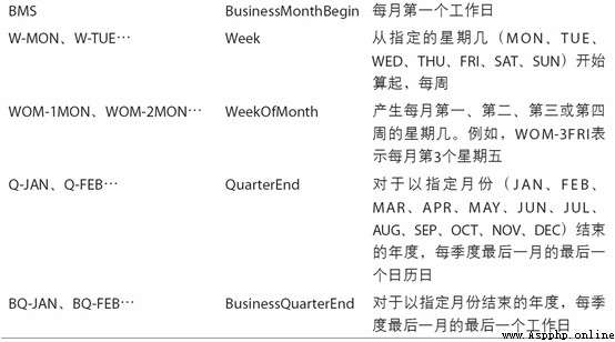
WOM(Week Of Month) Is a very practical frequency class , It uses WOM start . It enables you to get things like “ Every month 3 Next Friday ” Dates like that :
In [89]: rng = pd.date_range('2012-01-01', '2012-09-01', freq='WOM-3FRI')
In [90]: list(rng)
Out[90]:
[Timestamp('2012-01-20 00:00:00', freq='WOM-3FRI'),
Timestamp('2012-02-17 00:00:00', freq='WOM-3FRI'),
Timestamp('2012-03-16 00:00:00', freq='WOM-3FRI'),
Timestamp('2012-04-20 00:00:00', freq='WOM-3FRI'),
Timestamp('2012-05-18 00:00:00', freq='WOM-3FRI'),
Timestamp('2012-06-15 00:00:00', freq='WOM-3FRI'),
Timestamp('2012-07-20 00:00:00', freq='WOM-3FRI'),
Timestamp('2012-08-17 00:00:00', freq='WOM-3FRI')]
Move (shifting) Moving data forward or backward along the time axis .Series and DataFrame There is one. shift Method is used to perform a simple forward or backward operation , Keep index unchanged :
In [91]: ts = pd.Series(np.random.randn(4),
....: index=pd.date_range('1/1/2000', periods=4, freq='M'))
In [92]: ts
Out[92]:
2000-01-31 -0.066748
2000-02-29 0.838639
2000-03-31 -0.117388
2000-04-30 -0.517795
Freq: M, dtype: float64
In [93]: ts.shift(2)
Out[93]:
2000-01-31 NaN
2000-02-29 NaN
2000-03-31 -0.066748
2000-04-30 0.838639
Freq: M, dtype: float64
In [94]: ts.shift(-2)
Out[94]:
2000-01-31 -0.117388
2000-02-29 -0.517795
2000-03-31 NaN
2000-04-30 NaN
Freq: M, dtype: float64
When we move like this , Missing data will be generated before or after the time series .
shift Usually used to calculate a time series or multiple time series ( Such as DataFrame The column of ) Percentage change in . It can be expressed as :
ts / ts.shift(1) - 1
Because the simple shift operation will not modify the index , So some data will be discarded . therefore , If the frequency is known , It can be passed to shift In order to realize the displacement of the timestamp rather than the simple displacement of the data :
In [95]: ts.shift(2, freq='M')
Out[95]:
2000-03-31 -0.066748
2000-04-30 0.838639
2000-05-31 -0.117388
2000-06-30 -0.517795
Freq: M, dtype: float64
Other frequencies can also be used here , So you can flexibly process the data ahead and behind :
In [96]: ts.shift(3, freq='D')
Out[96]:
2000-02-03 -0.066748
2000-03-03 0.838639
2000-04-03 -0.117388
2000-05-03 -0.517795
dtype: float64
In [97]: ts.shift(1, freq='90T')
Out[97]:
2000-01-31 01:30:00 -0.066748
2000-02-29 01:30:00 0.838639
2000-03-31 01:30:00 -0.117388
2000-04-30 01:30:00 -0.517795
Freq: M, dtype: float64
pandas The date offset of can also be used in datetime or Timestamp On the object :
In [98]: from pandas.tseries.offsets import Day, MonthEnd
In [99]: now = datetime(2011, 11, 17)
In [100]: now + 3 * Day()
Out[100]: Timestamp('2011-11-20 00:00:00')
If you add anchor offset ( such as MonthEnd), The first increment scrolls the original date forward to the next date that meets the frequency rule :
In [101]: now + MonthEnd()
Out[101]: Timestamp('2011-11-30 00:00:00')
In [102]: now + MonthEnd(2)
Out[102]: Timestamp('2011-12-31 00:00:00')
Through the offset of the anchor rollforward and rollback Method , The date can be explicitly moved forward or backward “ rolling ”:
In [103]: offset = MonthEnd()
In [104]: offset.rollforward(now)
Out[104]: Timestamp('2011-11-30 00:00:00')
In [105]: offset.rollback(now)
Out[105]: Timestamp('2011-10-31 00:00:00')
There is another clever use of date offsets , That is to combine groupby Use these two “ rolling ” Method :
In [106]: ts = pd.Series(np.random.randn(20),
.....: index=pd.date_range('1/15/2000', periods=20, freq='4d'))
In [107]: ts
Out[107]:
2000-01-15 -0.116696
2000-01-19 2.389645
2000-01-23 -0.932454
2000-01-27 -0.229331
2000-01-31 -1.140330
2000-02-04 0.439920
2000-02-08 -0.823758
2000-02-12 -0.520930
2000-02-16 0.350282
2000-02-20 0.204395
2000-02-24 0.133445
2000-02-28 0.327905
2000-03-03 0.072153
2000-03-07 0.131678
2000-03-11 -1.297459
2000-03-15 0.997747
2000-03-19 0.870955
2000-03-23 -0.991253
2000-03-27 0.151699
2000-03-31 1.266151
Freq: 4D, dtype: float64
In [108]: ts.groupby(offset.rollforward).mean()
Out[108]:
2000-01-31 -0.005833
2000-02-29 0.015894
2000-03-31 0.150209
dtype: float64
Of course , It's simpler 、 A faster way to do this is to use resample(11.6 This is covered in detail in the section ):
In [109]: ts.resample('M').mean()
Out[109]:
2000-01-31 -0.005833
2000-02-29 0.015894
2000-03-31 0.150209
Freq: M, dtype: float64
The most annoying thing about time series processing is the processing of time zones . Many people choose to coordinate universal time (UTC, It's Greenwich mean time (Greenwich Mean Time) The replacement of , It is now an international standard ) To process time series . The time zone is in UTC In the form of an offset . for example , During daylight saving time , New York than UTC slow 4 Hours , At other times of the year UTC slow 5 Hours .
stay Python in , The time zone information comes from a third-party library pytz, It makes Python have access to Olson database ( Compiled world time zone information ). This is very important for historical data , This is because of various whims of local governments , Daylight saving time transition date ( even to the extent that UTC Offset ) There have been many changes . Take America for example ,DST The transition time is from 1900 It has changed many times since !
of pytz More information about the library , Please refer to its documentation . As far as this book is concerned , because pandas Packaged pytz The function of , So you don't have to remember API, Just remember the name of the time zone . The time zone name can be in shell see , It can also be viewed through the document :
In [110]: import pytz
In [111]: pytz.common_timezones[-5:]
Out[111]: ['US/Eastern', 'US/Hawaii', 'US/Mountain', 'US/Pacific', 'UTC']
From you to pytz Get the time zone object in , Use pytz.timezone that will do :
In [112]: tz = pytz.timezone('America/New_York')
In [113]: tz
Out[113]: <DstTzInfo 'America/New_York' LMT-1 day, 19:04:00 STD>
pandas The methods in can accept both time zone names and these objects .
By default ,pandas The time series in is simple (naive) The time zone . Take a look at this time series :
In [114]: rng = pd.date_range('3/9/2012 9:30', periods=6, freq='D')
In [115]: ts = pd.Series(np.random.randn(len(rng)), index=rng)
In [116]: ts
Out[116]:
2012-03-09 09:30:00 -0.202469
2012-03-10 09:30:00 0.050718
2012-03-11 09:30:00 0.639869
2012-03-12 09:30:00 0.597594
2012-03-13 09:30:00 -0.797246
2012-03-14 09:30:00 0.472879
Freq: D, dtype: float64
Its index is tz Field is None:
In [117]: print(ts.index.tz)
None
Date ranges can be generated from time zone sets :
In [118]: pd.date_range('3/9/2012 9:30', periods=10, freq='D', tz='UTC')
Out[118]:
DatetimeIndex(['2012-03-09 09:30:00+00:00', '2012-03-10 09:30:00+00:00',
'2012-03-11 09:30:00+00:00', '2012-03-12 09:30:00+00:00',
'2012-03-13 09:30:00+00:00', '2012-03-14 09:30:00+00:00',
'2012-03-15 09:30:00+00:00', '2012-03-16 09:30:00+00:00',
'2012-03-17 09:30:00+00:00', '2012-03-18 09:30:00+00:00'],
dtype='datetime64[ns, UTC]', freq='D')
The transformation from simplicity to localization is through tz_localize method-treated :
In [119]: ts
Out[119]:
2012-03-09 09:30:00 -0.202469
2012-03-10 09:30:00 0.050718
2012-03-11 09:30:00 0.639869
2012-03-12 09:30:00 0.597594
2012-03-13 09:30:00 -0.797246
2012-03-14 09:30:00 0.472879
Freq: D, dtype: float64
In [120]: ts_utc = ts.tz_localize('UTC')
In [121]: ts_utc
Out[121]:
2012-03-09 09:30:00+00:00 -0.202469
2012-03-10 09:30:00+00:00 0.050718
2012-03-11 09:30:00+00:00 0.639869
2012-03-12 09:30:00+00:00 0.597594
2012-03-13 09:30:00+00:00 -0.797246
2012-03-14 09:30:00+00:00 0.472879
Freq: D, dtype: float64
In [122]: ts_utc.index
Out[122]:
DatetimeIndex(['2012-03-09 09:30:00+00:00', '2012-03-10 09:30:00+00:00',
'2012-03-11 09:30:00+00:00', '2012-03-12 09:30:00+00:00',
'2012-03-13 09:30:00+00:00', '2012-03-14 09:30:00+00:00'],
dtype='datetime64[ns, UTC]', freq='D')
Once the time series are localized to a specific time zone , You can use it tz_convert It was transferred to another time zone :
In [123]: ts_utc.tz_convert('America/New_York')
Out[123]:
2012-03-09 04:30:00-05:00 -0.202469
2012-03-10 04:30:00-05:00 0.050718
2012-03-11 05:30:00-04:00 0.639869
2012-03-12 05:30:00-04:00 0.597594
2012-03-13 05:30:00-04:00 -0.797246
2012-03-14 05:30:00-04:00 0.472879
Freq: D, dtype: float64
For the above time series ( It spans the transition period of daylight saving time in the eastern time zone of the United States ), We can localize it to EST, And then convert to UTC Or Berlin time :
In [124]: ts_eastern = ts.tz_localize('America/New_York')
In [125]: ts_eastern.tz_convert('UTC')
Out[125]:
2012-03-09 14:30:00+00:00 -0.202469
2012-03-10 14:30:00+00:00 0.050718
2012-03-11 13:30:00+00:00 0.639869
2012-03-12 13:30:00+00:00 0.597594
2012-03-13 13:30:00+00:00 -0.797246
2012-03-14 13:30:00+00:00 0.472879
Freq: D, dtype: float64
In [126]: ts_eastern.tz_convert('Europe/Berlin')
Out[126]:
2012-03-09 15:30:00+01:00 -0.202469
2012-03-10 15:30:00+01:00 0.050718
2012-03-11 14:30:00+01:00 0.639869
2012-03-12 14:30:00+01:00 0.597594
2012-03-13 14:30:00+01:00 -0.797246
2012-03-14 14:30:00+01:00 0.472879
Freq: D, dtype: float64
tz_localize and tz_convert It's also DatetimeIndex Instance method of :
In [127]: ts.index.tz_localize('Asia/Shanghai')
Out[127]:
DatetimeIndex(['2012-03-09 09:30:00+08:00', '2012-03-10 09:30:00+08:00',
'2012-03-11 09:30:00+08:00', '2012-03-12 09:30:00+08:00',
'2012-03-13 09:30:00+08:00', '2012-03-14 09:30:00+08:00'],
dtype='datetime64[ns, Asia/Shanghai]', freq='D')
Be careful : Localizing a simple timestamp also checks for times that are easily confused or do not exist near the daylight saving time transition period .
Similar to time series and date ranges , independent Timestamp Objects can also be transformed from simplex (naive) Localize to time zone aware (time zone-aware), And switch from one time zone to another :
In [128]: stamp = pd.Timestamp('2011-03-12 04:00')
In [129]: stamp_utc = stamp.tz_localize('utc')
In [130]: stamp_utc.tz_convert('America/New_York')
Out[130]: Timestamp('2011-03-11 23:00:00-0500', tz='America/New_York')
Creating Timestamp when , You can also pass in a time zone information :
In [131]: stamp_moscow = pd.Timestamp('2011-03-12 04:00', tz='Europe/Moscow')
In [132]: stamp_moscow
Out[132]: Timestamp('2011-03-12 04:00:00+0300', tz='Europe/Moscow')
Time zone conscious Timestamp Object internally holds a UTC Timestamp value ( since UNIX An era (1970 year 1 month 1 Japan ) The number of nanoseconds counted ). This UTC Values do not change during time zone conversion :
In [133]: stamp_utc.value
Out[133]: 1299902400000000000
In [134]: stamp_utc.tz_convert('America/New_York').value
Out[134]: 1299902400000000000
When using pandas Of DateOffset Object to perform time arithmetic operations , The calculation process will automatically focus on whether there is a daylight saving time transition period . here , We created in DST The timestamp before the transition . First , Take a look at what happened before daylight saving time 30 minute :
In [135]: from pandas.tseries.offsets import Hour
In [136]: stamp = pd.Timestamp('2012-03-12 01:30', tz='US/Eastern')
In [137]: stamp
Out[137]: Timestamp('2012-03-12 01:30:00-0400', tz='US/Eastern')
In [138]: stamp + Hour()
Out[138]: Timestamp('2012-03-12 02:30:00-0400', tz='US/Eastern')
then , Before daylight saving time 90 minute :
In [139]: stamp = pd.Timestamp('2012-11-04 00:30', tz='US/Eastern')
In [140]: stamp
Out[140]: Timestamp('2012-11-04 00:30:00-0400', tz='US/Eastern')
In [141]: stamp + 2 * Hour()
Out[141]: Timestamp('2012-11-04 01:30:00-0500', tz='US/Eastern')
If the time zones of two time series are different , When you merge them together , The end result will be UTC. Because the time stamp is actually UTC Stored , So this is a very simple operation , No conversion is required :
In [142]: rng = pd.date_range('3/7/2012 9:30', periods=10, freq='B')
In [143]: ts = pd.Series(np.random.randn(len(rng)), index=rng)
In [144]: ts
Out[144]:
2012-03-07 09:30:00 0.522356
2012-03-08 09:30:00 -0.546348
2012-03-09 09:30:00 -0.733537
2012-03-12 09:30:00 1.302736
2012-03-13 09:30:00 0.022199
2012-03-14 09:30:00 0.364287
2012-03-15 09:30:00 -0.922839
2012-03-16 09:30:00 0.312656
2012-03-19 09:30:00 -1.128497
2012-03-20 09:30:00 -0.333488
Freq: B, dtype: float64
In [145]: ts1 = ts[:7].tz_localize('Europe/London')
In [146]: ts2 = ts1[2:].tz_convert('Europe/Moscow')
In [147]: result = ts1 + ts2
In [148]: result.index
Out[148]:
DatetimeIndex(['2012-03-07 09:30:00+00:00', '2012-03-08 09:30:00+00:00',
'2012-03-09 09:30:00+00:00', '2012-03-12 09:30:00+00:00',
'2012-03-13 09:30:00+00:00', '2012-03-14 09:30:00+00:00',
'2012-03-15 09:30:00+00:00'],
dtype='datetime64[ns, UTC]', freq='B')
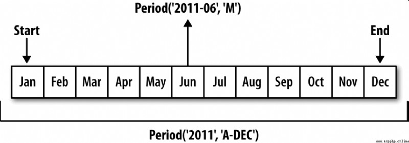
period (period) It's a time interval , For example, a few days 、 Months 、 Several seasons 、 Years and so on .Period Class represents this data type , Its constructor needs to use a string or integer , And the watch 11-4 The frequency in :
In [149]: p = pd.Period(2007, freq='A-DEC')
In [150]: p
Out[150]: Period('2007', 'A-DEC')
here , This Period Object represents from 2007 year 1 month 1 The day is coming 2007 year 12 month 31 The whole time between days . Only need to Period The object can be shifted according to its frequency by adding or subtracting an integer :
In [151]: p + 5
Out[151]: Period('2012', 'A-DEC')
In [152]: p - 2
Out[152]: Period('2005', 'A-DEC')
If two Period Objects have the same frequency , Then the difference is the number of units between them :
In [153]: pd.Period('2014', freq='A-DEC') - p
Out[153]: 7
period_range Function can be used to create a period range of rules :
In [154]: rng = pd.period_range('2000-01-01', '2000-06-30', freq='M')
In [155]: rng
Out[155]: PeriodIndex(['2000-01', '2000-02', '2000-03', '2000-04', '2000-05', '20
00-06'], dtype='period[M]', freq='M')
PeriodIndex Class holds a set of Period, It can be in any pandas Used as axis index in data structure :
In [156]: pd.Series(np.random.randn(6), index=rng)
Out[156]:
2000-01 -0.514551
2000-02 -0.559782
2000-03 -0.783408
2000-04 -1.797685
2000-05 -0.172670
2000-06 0.680215
Freq: M, dtype: float64
If you have an array of strings , You can also use PeriodIndex class :
In [157]: values = ['2001Q3', '2002Q2', '2003Q1']
In [158]: index = pd.PeriodIndex(values, freq='Q-DEC')
In [159]: index
Out[159]: PeriodIndex(['2001Q3', '2002Q2', '2003Q1'], dtype='period[Q-DEC]', freq
='Q-DEC')
Period and PeriodIndex Objects can be accessed through their asfreq Methods are converted to other frequencies . Suppose we have an annual period , Hope to convert it to a monthly period at the beginning or end of the year . The task is very simple :
In [160]: p = pd.Period('2007', freq='A-DEC')
In [161]: p
Out[161]: Period('2007', 'A-DEC')
In [162]: p.asfreq('M', how='start')
Out[162]: Period('2007-01', 'M')
In [163]: p.asfreq('M', how='end')
Out[163]: Period('2007-12', 'M')
You can take Period(‘2007’,‘A-DEC’) Think of it as a cursor in a time period divided into multiple monthly periods . chart 11-1 This is explained . For a person who does not 12 The fiscal year ending in December , The attribution of monthly sub periods is different :
In [164]: p = pd.Period('2007', freq='A-JUN')
In [165]: p
Out[165]: Period('2007', 'A-JUN')
In [166]: p.asfreq('M', 'start')
Out[166]: Period('2006-07', 'M')
In [167]: p.asfreq('M', 'end')
Out[167]: Period('2007-06', 'M')
When converting high frequency to low frequency , Over time (superperiod) It's from the period of Zi (subperiod) It's decided by the location of the place . for example , stay A-JUN Medium frequency , month “2007 year 8 month ” It's actually a cycle “2008 year ” Of :
In [168]: p = pd.Period('Aug-2007', 'M')
In [169]: p.asfreq('A-JUN')
Out[169]: Period('2008', 'A-JUN')
complete PeriodIndex or TimeSeries The same is true of the frequency conversion mode :
In [170]: rng = pd.period_range('2006', '2009', freq='A-DEC')
In [171]: ts = pd.Series(np.random.randn(len(rng)), index=rng)
In [172]: ts
Out[172]:
2006 1.607578
2007 0.200381
2008 -0.834068
2009 -0.302988
Freq: A-DEC, dtype: float64
In [173]: ts.asfreq('M', how='start')
Out[173]:
2006-01 1.607578
2007-01 0.200381
2008-01 -0.834068
2009-01 -0.302988
Freq: M, dtype: float64
here , According to the first month of the year period , The annual period is replaced by the monthly period . If we want the last working day of the year , We can use “B” frequency , And indicate the end of the period :
In [174]: ts.asfreq('B', how='end')
Out[174]:
2006-12-29 1.607578
2007-12-31 0.200381
2008-12-31 -0.834068
2009-12-31 -0.302988
Freq: B, dtype: float64
Quarterly data in accounting 、 It is very common in fields such as finance . A lot of quarterly data will involve “ End of financial year ” The concept of , It's usually a year 12 The last calendar day or working day of a month in a month . At this point , period "2012Q4" It has different meanings according to the end of the financial year .pandas Support 12 Possible quarterly frequencies , namely Q-JAN To Q-DEC:
In [175]: p = pd.Period('2012Q4', freq='Q-JAN')
In [176]: p
Out[176]: Period('2012Q4', 'Q-JAN')
In order to 1 In the fiscal year ending in December ,2012Q4 It's from 11 Month to 1 month ( It will be clear if you convert it into Japanese frequency ). chart 11-2 This is explained :
In [177]: p.asfreq('D', 'start')
Out[177]: Period('2011-11-01', 'D')
In [178]: p.asfreq('D', 'end')
Out[178]: Period('2012-01-31', 'D')
therefore ,Period The arithmetic operation between them will be very simple . for example , To get the penultimate business day afternoon of the quarter 4 Time stamp of the point , You can do this :
In [179]: p4pm = (p.asfreq('B', 'e') - 1).asfreq('T', 's') + 16 * 60
In [180]: p4pm
Out[180]: Period('2012-01-30 16:00', 'T')
In [181]: p4pm.to_timestamp()
Out[181]: Timestamp('2012-01-30 16:00:00')
period_range Can be used to generate quarterly ranges . The arithmetic operation of the quarterly range is the same as above :
In [182]: rng = pd.period_range('2011Q3', '2012Q4', freq='Q-JAN')
In [183]: ts = pd.Series(np.arange(len(rng)), index=rng)
In [184]: ts
Out[184]:
2011Q3 0
2011Q4 1
2012Q1 2
2012Q2 3
2012Q3 4
2012Q4 5
Freq: Q-JAN, dtype: int64
In [185]: new_rng = (rng.asfreq('B', 'e') - 1).asfreq('T', 's') + 16 * 60
In [186]: ts.index = new_rng.to_timestamp()
In [187]: ts
Out[187]:
2010-10-28 16:00:00 0
2011-01-28 16:00:00 1
2011-04-28 16:00:00 2
2011-07-28 16:00:00 3
2011-10-28 16:00:00 4
2012-01-30 16:00:00 5
dtype: int64
By using to_period Method , Can be indexed by a timestamp Series and DataFrame Object to index by period :
In [188]: rng = pd.date_range('2000-01-01', periods=3, freq='M')
In [189]: ts = pd.Series(np.random.randn(3), index=rng)
In [190]: ts
Out[190]:
2000-01-31 1.663261
2000-02-29 -0.996206
2000-03-31 1.521760
Freq: M, dtype: float64
In [191]: pts = ts.to_period()
In [192]: pts
Out[192]:
2000-01 1.663261
2000-02 -0.996206
2000-03 1.521760
Freq: M, dtype: float64
Since periods refer to non overlapping time intervals , So for a given frequency , A timestamp can only belong to one period . new PeriodIndex The default frequency of is inferred from the timestamp , You can also specify any other frequency . Repeated periods are allowed in the results :
In [193]: rng = pd.date_range('1/29/2000', periods=6, freq='D')
In [194]: ts2 = pd.Series(np.random.randn(6), index=rng)
In [195]: ts2
Out[195]:
2000-01-29 0.244175
2000-01-30 0.423331
2000-01-31 -0.654040
2000-02-01 2.089154
2000-02-02 -0.060220
2000-02-03 -0.167933
Freq: D, dtype: float64
In [196]: ts2.to_period('M')
Out[196]:
2000-01 0.244175
2000-01 0.423331
2000-01 -0.654040
2000-02 2.089154
2000-02 -0.060220
2000-02 -0.167933
Freq: M, dtype: float64
To convert back to a timestamp , Use to_timestamp that will do :
In [197]: pts = ts2.to_period()
In [198]: pts
Out[198]:
2000-01-29 0.244175
2000-01-30 0.423331
2000-01-31 -0.654040
2000-02-01 2.089154
2000-02-02 -0.060220
2000-02-03 -0.167933
Freq: D, dtype: float64
In [199]: pts.to_timestamp(how='end')
Out[199]:
2000-01-29 0.244175
2000-01-30 0.423331
2000-01-31 -0.654040
2000-02-01 2.089154
2000-02-02 -0.060220
2000-02-03 -0.167933
Freq: D, dtype: float64
Fixed frequency data sets usually store time information in multiple columns . for example , In the following macroeconomic data set , The year and quarter are stored in different columns :
In [200]: data = pd.read_csv('examples/macrodata.csv')
In [201]: data.head(5)
Out[201]:
year quarter realgdp realcons realinv realgovt realdpi cpi \
0 1959.0 1.0 2710.349 1707.4 286.898 470.045 1886.9 28.98
1 1959.0 2.0 2778.801 1733.7 310.859 481.301 1919.7 29.15
2 1959.0 3.0 2775.488 1751.8 289.226 491.260 1916.4 29.35
3 1959.0 4.0 2785.204 1753.7 299.356 484.052 1931.3 29.37
4 1960.0 1.0 2847.699 1770.5 331.722 462.199 1955.5 29.54
m1 tbilrate unemp pop infl realint
0 139.7 2.82 5.8 177.146 0.00 0.00
1 141.7 3.08 5.1 177.830 2.34 0.74
2 140.5 3.82 5.3 178.657 2.74 1.09
3 140.0 4.33 5.6 179.386 0.27 4.06
4 139.6 3.50 5.2 180.007 2.31 1.19
In [202]: data.year
Out[202]:
0 1959.0
1 1959.0
2 1959.0
3 1959.0
4 1960.0
5 1960.0
6 1960.0
7 1960.0
8 1961.0
9 1961.0
...
193 2007.0
194 2007.0
195 2007.0
196 2008.0
197 2008.0
198 2008.0
199 2008.0
200 2009.0
201 2009.0
202 2009.0
Name: year, Length: 203, dtype: float64
In [203]: data.quarter
Out[203]:
0 1.0
1 2.0
2 3.0
3 4.0
4 1.0
5 2.0
6 3.0
7 4.0
8 1.0
9 2.0
...
193 2.0
194 3.0
195 4.0
196 1.0
197 2.0
198 3.0
199 4.0
200 1.0
201 2.0
202 3.0
Name: quarter, Length: 203, dtype: float64
By passing these arrays and a frequency into PeriodIndex, You can merge them into DataFrame An index of :
In [204]: index = pd.PeriodIndex(year=data.year, quarter=data.quarter,
.....: freq='Q-DEC')
In [205]: index
Out[205]:
PeriodIndex(['1959Q1', '1959Q2', '1959Q3', '1959Q4', '1960Q1', '1960Q2',
'1960Q3', '1960Q4', '1961Q1', '1961Q2',
...
'2007Q2', '2007Q3', '2007Q4', '2008Q1', '2008Q2', '2008Q3',
'2008Q4', '2009Q1', '2009Q2', '2009Q3'],
dtype='period[Q-DEC]', length=203, freq='Q-DEC')
In [206]: data.index = index
In [207]: data.infl
Out[207]:
1959Q1 0.00
1959Q2 2.34
1959Q3 2.74
1959Q4 0.27
1960Q1 2.31
1960Q2 0.14
1960Q3 2.70
1960Q4 1.21
1961Q1 -0.40
1961Q2 1.47
...
2007Q2 2.75
2007Q3 3.45
2007Q4 6.38
2008Q1 2.82
2008Q2 8.53
2008Q3 -3.16
2008Q4 -8.79
2009Q1 0.94
2009Q2 3.37
2009Q3 3.56
Freq: Q-DEC, Name: infl, Length: 203, dtype: float64
Resampling (resampling) It refers to the process of converting time series from one frequency to another . Aggregating high-frequency data to low-frequency data is called downsampling (downsampling), Converting low-frequency data to high-frequency data is called up sampling (upsampling). Not all resampling can be divided into these two categories . for example , take W-WED( Three days a week ) Convert to W-FRI Neither downsampling nor upsampling .
pandas Objects all have a resample Method , It is the main function of all kinds of frequency conversion .resample There's a similar one groupby Of API, call resample You can group data , Then an aggregate function is called :
In [208]: rng = pd.date_range('2000-01-01', periods=100, freq='D')
In [209]: ts = pd.Series(np.random.randn(len(rng)), index=rng)
In [210]: ts
Out[210]:
2000-01-01 0.631634
2000-01-02 -1.594313
2000-01-03 -1.519937
2000-01-04 1.108752
2000-01-05 1.255853
2000-01-06 -0.024330
2000-01-07 -2.047939
2000-01-08 -0.272657
2000-01-09 -1.692615
2000-01-10 1.423830
...
2000-03-31 -0.007852
2000-04-01 -1.638806
2000-04-02 1.401227
2000-04-03 1.758539
2000-04-04 0.628932
2000-04-05 -0.423776
2000-04-06 0.789740
2000-04-07 0.937568
2000-04-08 -2.253294
2000-04-09 -1.772919
Freq: D, Length: 100, dtype: float64
In [211]: ts.resample('M').mean()
Out[211]:
2000-01-31 -0.165893
2000-02-29 0.078606
2000-03-31 0.223811
2000-04-30 -0.063643
Freq: M, dtype: float64
In [212]: ts.resample('M', kind='period').mean()
Out[212]:
2000-01 -0.165893
2000-02 0.078606
2000-03 0.223811
2000-04 -0.063643
Freq: M, dtype: float64
resample Is a flexible and efficient method , It can be used to deal with very large time series . I will illustrate its usage through a series of examples . surface 11-5 Summarize some of its options .
surface 11-5 resample Method parameters 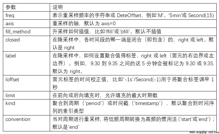
Aggregating data into regular low frequencies is a very common time series processing task . The data to be aggregated does not have to have a fixed frequency , The desired frequency will automatically define the aggregated bin boundary , These facets are used to split the time series into multiple segments . for example , To switch to monthly frequency (‘M’ or ’BM’), The data needs to be divided into multiple single month time periods . All time periods are semi open . A data point can only belong to one time period , The union of all time periods must be able to form the whole time frame . In use resample When downsampling data , Two things need to be considered :
To illustrate , Let's take a look at some “1 minute ” data :
In [213]: rng = pd.date_range('2000-01-01', periods=12, freq='T')
In [214]: ts = pd.Series(np.arange(12), index=rng)
In [215]: ts
Out[215]:
2000-01-01 00:00:00 0
2000-01-01 00:01:00 1
2000-01-01 00:02:00 2
2000-01-01 00:03:00 3
2000-01-01 00:04:00 4
2000-01-01 00:05:00 5
2000-01-01 00:06:00 6
2000-01-01 00:07:00 7
2000-01-01 00:08:00 8
2000-01-01 00:09:00 9
2000-01-01 00:10:00 10
2000-01-01 00:11:00 11
Freq: T, dtype: int64
Suppose you want to aggregate these data into by summation “5 minute ” In block :
In [216]: ts.resample('5min', closed='right').sum()
Out[216]:
1999-12-31 23:55:00 0
2000-01-01 00:00:00 15
2000-01-01 00:05:00 40
2000-01-01 00:10:00 11
Freq: 5T, dtype: int64
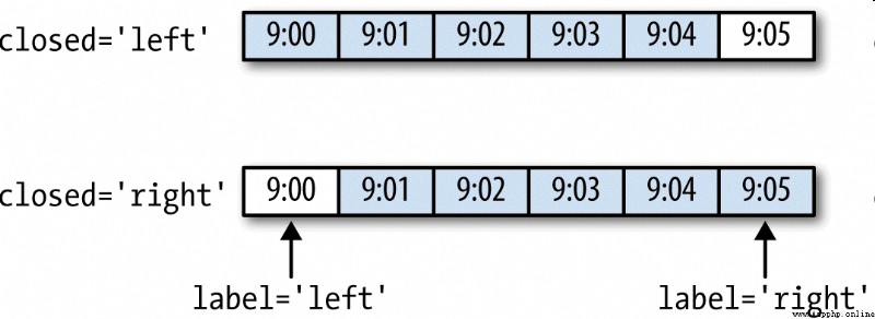
The incoming frequency will be in “5 minute ” The increment of defines the boundary of the panel . By default , The right boundary of the bin is inclusive , therefore 00:00 To 00:05 The interval of contains 00:05 Of . Pass in closed='left’ Will close the interval with the left boundary :
In [217]: ts.resample('5min', closed='right').sum()
Out[217]:
1999-12-31 23:55:00 0
2000-01-01 00:00:00 15
2000-01-01 00:05:00 40
2000-01-01 00:10:00 11
Freq: 5T, dtype: int64
As you can see , The final time series is marked with the timestamp of the right boundary of each bin . Pass in label='right’ That is, a bin can be marked by its postcode boundary :
In [218]: ts.resample('5min', closed='right', label='right').sum()
Out[218]:
2000-01-01 00:00:00 0
2000-01-01 00:05:00 15
2000-01-01 00:10:00 40
2000-01-01 00:15:00 11
Freq: 5T, dtype: int64
chart 11-3 Illustrates the “1 minute ” The data is converted to “5 minute ” Data processing process .
Last , You may want to do some displacement on the result index , For example, subtract one second from the right boundary to make it easier to understand which interval the timestamp represents . Just pass loffset You can do this by setting a string or date offset :
In [219]: ts.resample('5min', closed='right',
.....: label='right', loffset='-1s').sum()
Out[219]:
1999-12-31 23:59:59 0
2000-01-01 00:04:59 15
In [219]: ts.resample('5min', closed='right',
.....: label='right', loffset='-1s').sum()
Out[219]:
1999-12-31 23:59:59 0
2000-01-01 00:04:59 15
Besides , You can also call the... Of the result object shift Method to achieve this , So there's no need to set up loffset 了 .
##OHLC Resampling
There is an omnipresent way of time series aggregation in the financial field , That is, calculate the four values of each bin : The first value is (open, The opening quotation )、 Last value (close, The close )、 Maximum (high, The highest ) And the minimum (low, The minimum ). Pass in how='ohlc’ You can get a with these four aggregate values DataFrame. The whole process is efficient , Only one scan is needed to calculate the result :
In [220]: ts.resample('5min').ohlc()
Out[220]:
open high low close
2000-01-01 00:00:00 0 4 0 4
2000-01-01 00:05:00 5 9 5 9
2000-01-01 00:10:00 10 11 10 11
## Upsampling and interpolation
When converting data from low frequency to high frequency , There is no need for aggregation . Let's look at a with some weekly data DataFrame:
In [221]: frame = pd.DataFrame(np.random.randn(2, 4),
.....: index=pd.date_range('1/1/2000', periods=2,
.....: freq='W-WED'),
.....: columns=['Colorado', 'Texas', 'New York', 'Ohio'])
In [222]: frame
Out[222]:
Colorado Texas New York Ohio
2000-01-05 -0.896431 0.677263 0.036503 0.087102
2000-01-12 -0.046662 0.927238 0.482284 -0.867130
When you aggregate this data , There is only one value per group , This introduces missing values . We use asfreq Method to convert to high frequency , Without polymerization :
In [223]: df_daily = frame.resample('D').asfreq()
In [224]: df_daily
Out[224]:
Colorado Texas New York Ohio
2000-01-05 -0.896431 0.677263 0.036503 0.087102
2000-01-06 NaN NaN NaN NaN
2000-01-07 NaN NaN NaN NaN
2000-01-08 NaN NaN NaN NaN
2000-01-09 NaN NaN NaN NaN
2000-01-10 NaN NaN NaN NaN
2000-01-11 NaN NaN NaN NaN
2000-01-12 -0.046662 0.927238 0.482284 -0.867130
Suppose you want to fill in with the previous week values “ Non Wednesday ”.resampling The filling and interpolation methods of are the same as fillna and reindex The same as :
In [225]: frame.resample('D').ffill()
Out[225]:
Colorado Texas New York Ohio
2000-01-05 -0.896431 0.677263 0.036503 0.087102
2000-01-06 -0.896431 0.677263 0.036503 0.087102
2000-01-07 -0.896431 0.677263 0.036503 0.087102
2000-01-08 -0.896431 0.677263 0.036503 0.087102
2000-01-09 -0.896431 0.677263 0.036503 0.087102
2000-01-10 -0.896431 0.677263 0.036503 0.087102
2000-01-11 -0.896431 0.677263 0.036503 0.087102
2000-01-12 -0.046662 0.927238 0.482284 -0.867130
Again , You can also fill in only the specified number of periods ( The aim is to limit the continuous use distance of previous observations ):
In [226]: frame.resample('D').ffill(limit=2)
Out[226]:
Colorado Texas New York Ohio
2000-01-05 -0.896431 0.677263 0.036503 0.087102
2000-01-06 -0.896431 0.677263 0.036503 0.087102
2000-01-07 -0.896431 0.677263 0.036503 0.087102
2000-01-08 NaN NaN NaN NaN
2000-01-09 NaN NaN NaN NaN
2000-01-10 NaN NaN NaN NaN
2000-01-11 NaN NaN NaN NaN
2000-01-12 -0.046662 0.927238 0.482284 -0.867130
Be careful , There is no need for the new date index to overlap with the old one :
In [227]: frame.resample('W-THU').ffill()
Out[227]:
Colorado Texas New York Ohio
2000-01-06 -0.896431 0.677263 0.036503 0.087102
2000-01-13 -0.046662 0.927238 0.482284 -0.867130
Resampling data that uses a period index is much like a timestamp :
In [228]: frame = pd.DataFrame(np.random.randn(24, 4),
.....: index=pd.period_range('1-2000', '12-2001',
.....: freq='M'),
.....: columns=['Colorado', 'Texas', 'New York', 'Ohio'])
In [229]: frame[:5]
Out[229]:
Colorado Texas New York Ohio
2000-01 0.493841 -0.155434 1.397286 1.507055
2000-02 -1.179442 0.443171 1.395676 -0.529658
2000-03 0.787358 0.248845 0.743239 1.267746
2000-04 1.302395 -0.272154 -0.051532 -0.467740
2000-05 -1.040816 0.426419 0.312945 -1.115689
In [230]: annual_frame = frame.resample('A-DEC').mean()
In [231]: annual_frame
Out[231]:
Colorado Texas New York Ohio
2000 0.556703 0.016631 0.111873 -0.027445
2001 0.046303 0.163344 0.251503 -0.157276
It's a little bit more troublesome , Because you have to decide which end of each interval in the new frequency is used to place the original value , It's like asfreq In that way .convention The parameter defaults to ’start’, It can also be set to ’end’:
# Q-DEC: Quarterly, year ending in December
In [232]: annual_frame.resample('Q-DEC').ffill()
Out[232]:
Colorado Texas New York Ohio
2000Q1 0.556703 0.016631 0.111873 -0.027445
2000Q2 0.556703 0.016631 0.111873 -0.027445
2000Q3 0.556703 0.016631 0.111873 -0.027445
2000Q4 0.556703 0.016631 0.111873 -0.027445
2001Q1 0.046303 0.163344 0.251503 -0.157276
2001Q2 0.046303 0.163344 0.251503 -0.157276
2001Q3 0.046303 0.163344 0.251503 -0.157276
2001Q4 0.046303 0.163344 0.251503 -0.157276
In [233]: annual_frame.resample('Q-DEC', convention='end').ffill()
Out[233]:
Colorado Texas New York Ohio
2000Q4 0.556703 0.016631 0.111873 -0.027445
2001Q1 0.556703 0.016631 0.111873 -0.027445
2001Q2 0.556703 0.016631 0.111873 -0.027445
2001Q3 0.556703 0.016631 0.111873 -0.027445
2001Q4 0.046303 0.163344 0.251503 -0.157276
Because period refers to time interval , So the rules of upsampling and downsampling are relatively strict :
If these conditions are not met , It will cause an exception . This mainly affects the seasonal 、 year 、 Frequency of weekly calculation . for example , from Q-MAR The defined time interval can only be upsampled to A-MAR、A-JUN、A-SEP、A-DEC etc. :
In [234]: annual_frame.resample('Q-MAR').ffill()
Out[234]:
Colorado Texas New York Ohio
2000Q4 0.556703 0.016631 0.111873 -0.027445
2001Q1 0.556703 0.016631 0.111873 -0.027445
2001Q2 0.556703 0.016631 0.111873 -0.027445
2001Q3 0.556703 0.016631 0.111873 -0.027445
2001Q4 0.046303 0.163344 0.251503 -0.157276
2002Q1 0.046303 0.163344 0.251503 -0.157276
2002Q2 0.046303 0.163344 0.251503 -0.157276
2002Q3 0.046303 0.163344 0.251503 -0.157276
Moving windows ( Can have exponential decay weights ) The various statistical functions calculated on are also a kind of array transformation commonly used in time series . In this way, noise data or fracture data can be smoothed . I call them the move window function (moving window function), It also includes functions with variable window lengths ( Such as exponentially weighted moving average ). Like other statistical functions , The move window function will also automatically exclude missing values .
Before the start , We load some time series data , Resample it to weekday frequency :
In [235]: close_px_all = pd.read_csv('examples/stock_px_2.csv',
.....: parse_dates=True, index_col=0)
In [236]: close_px = close_px_all[['AAPL', 'MSFT', 'XOM']]
In [237]: close_px = close_px.resample('B').ffill()
Now introduce rolling Operator , It is associated with resample and groupby It's like . Can be in TimeSeries or DataFrame And one. window( Indicates the number of periods , See the picture 11-4) Call it :
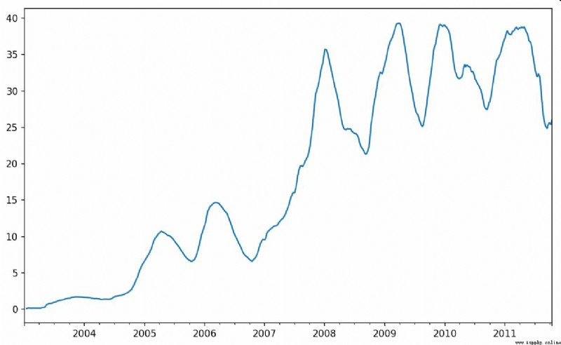
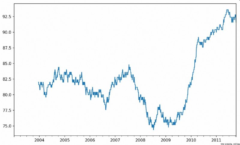
In [238]: close_px.AAPL.plot()
Out[238]: <matplotlib.axes._subplots.AxesSubplot at 0x7f2f2570cf98>
In [239]: close_px.AAPL.rolling(250).mean().plot()
expression rolling(250) And groupby It's like , But not grouped , Instead, create one that follows 250 Sliding window objects grouped by days . then , We get the price of Apple's stock 250 Day's mobile window .
By default ,rolling The function requires all values in the window to be non NA value . This behavior can be modified to solve the problem of missing data . Actually , The data that is not in the window period at the beginning of the time series is a special case ( See the picture 11-5):
In [241]: appl_std250 = close_px.AAPL.rolling(250, min_periods=10).std()
In [242]: appl_std250[5:12]
Out[242]:
2003-01-09 NaN
2003-01-10 NaN
2003-01-13 NaN
2003-01-14 NaN
2003-01-15 0.077496
2003-01-16 0.074760
2003-01-17 0.112368
Freq: B, Name: AAPL, dtype: float64
In [243]: appl_std250.plot()
To calculate the extended window average (expanding window mean), have access to expanding instead of rolling.“ Expand ” signify , Start the window from the beginning of the time series , Increase the window until it exceeds all the sequences .apple_std250 The extended window average of the time series is as follows :
In [244]: expanding_mean = appl_std250.expanding().mean()
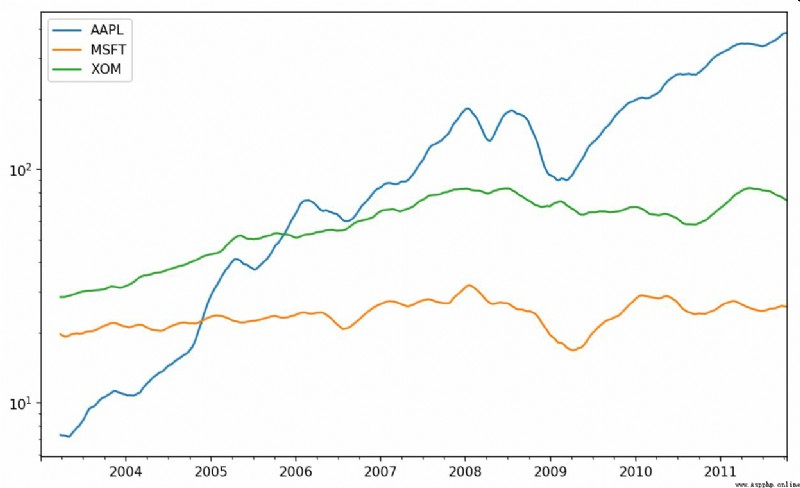
Yes DataFrame call rolling_mean( And similar functions ) The transformation will be applied to all columns ( See the picture 11-6):
In [246]: close_px.rolling(60).mean().plot(logy=True)
rolling Function can also accept a specified fixed size time compensation string , Not a set of periods . This makes it easy to deal with irregular time series . These strings can also be passed to resample. for example , We can calculate 20 Rolling average of days , As shown below :
In [247]: close_px.rolling('20D').mean()
Out[247]:
AAPL MSFT XOM
2003-01-02 7.400000 21.110000 29.220000
2003-01-03 7.425000 21.125000 29.230000
2003-01-06 7.433333 21.256667 29.473333
2003-01-07 7.432500 21.425000 29.342500
2003-01-08 7.402000 21.402000 29.240000
2003-01-09 7.391667 21.490000 29.273333
2003-01-10 7.387143 21.558571 29.238571
2003-01-13 7.378750 21.633750 29.197500
2003-01-14 7.370000 21.717778 29.194444
2003-01-15 7.355000 21.757000 29.152000
... ... ... ...
2011-10-03 398.002143 25.890714 72.413571
2011-10-04 396.802143 25.807857 72.427143
2011-10-05 395.751429 25.729286 72.422857
2011-10-06 394.099286 25.673571 72.375714
2011-10-07 392.479333 25.712000 72.454667
2011-10-10 389.351429 25.602143 72.527857
2011-10-11 388.505000 25.674286 72.835000
2011-10-12 388.531429 25.810000 73.400714
2011-10-13 388.826429 25.961429 73.905000
2011-10-14 391.038000 26.048667 74.185333
[2292 rows x 3 columns]
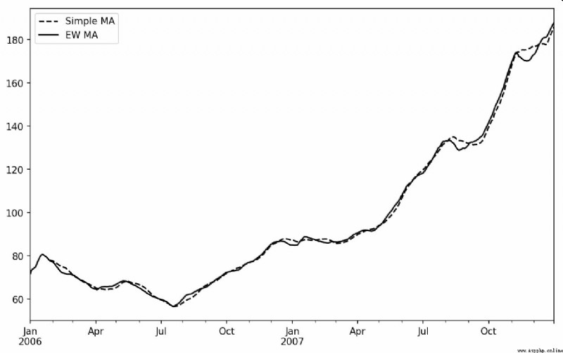
Another way to use fixed size windows and equal weight observations is , Define an attenuation factor (decay factor) Constant , So that the recent observations have a greater weight . There are many ways to define the attenuation factor , More popular is the use of time intervals (span), It makes the results compatible with simple moving windows whose window size is equal to the time interval (simple moving window) function .
Because exponential weighted statistics will give a greater weight to recent observations , So relative to the equal weight statistics , It can “ To adapt to ” Faster change .
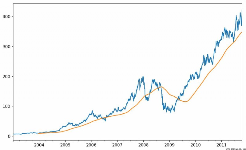
except rolling and expanding,pandas also ewm Operator . The following example compares Apple's share price 30 Daily moving average sum span=30 The exponentially weighted moving average of ( Pictured 11-7 Shown ):
In [249]: aapl_px = close_px.AAPL['2006':'2007']
In [250]: ma60 = aapl_px.rolling(30, min_periods=20).mean()
In [251]: ewma60 = aapl_px.ewm(span=30).mean()
In [252]: ma60.plot(style='k--', label='Simple MA')
Out[252]: <matplotlib.axes._subplots.AxesSubplot at 0x7f2f252161d0>
In [253]: ewma60.plot(style='k-', label='EW MA')
Out[253]: <matplotlib.axes._subplots.AxesSubplot at 0x7f2f252161d0>
In [254]: plt.legend()
Some statistical operations ( Such as correlation coefficient and covariance ) You need to execute on two time series . for example , Financial analysts often compare a stock to a reference index ( Such as standard & Poor's 500 Index ) Of interest . Explain , We first calculate the percentage change of the time series we are interested in :
In [256]: spx_px = close_px_all['SPX']
In [257]: spx_rets = spx_px.pct_change()
In [258]: returns = close_px.pct_change()
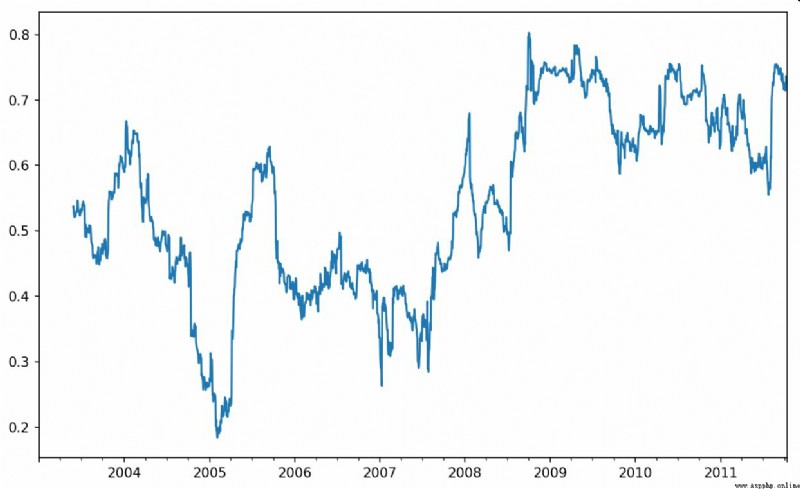
call rolling after ,corr The aggregate function begins to evaluate with spx_rets Rolling correlation coefficient ( The results are shown in the figure 11-8):
In [259]: corr = returns.AAPL.rolling(125, min_periods=100).corr(spx_rets)
In [260]: corr.plot()
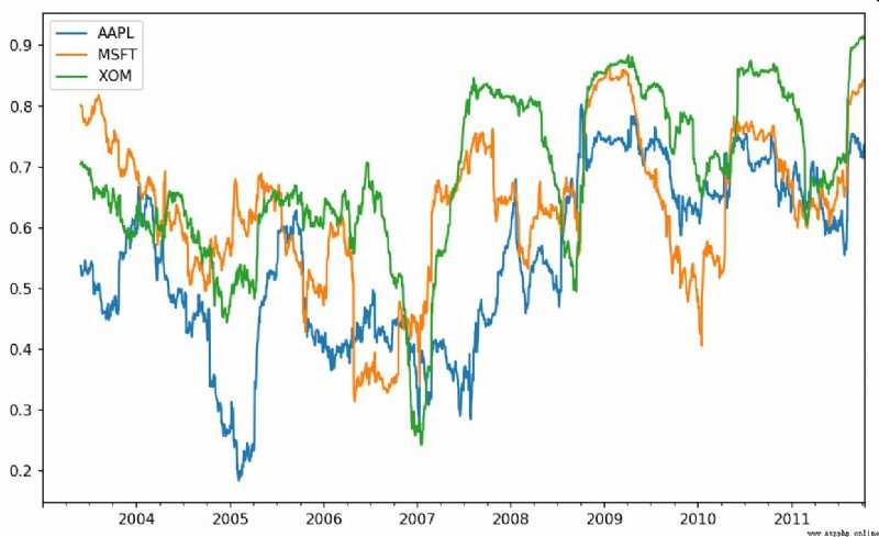
Suppose you want to calculate multiple stocks and S & P at one time 500 The correlation coefficient of the index . Write a loop and create a new one DataFrame It's not that hard , But it's wordy . Actually , Just pass in a TimeSeries And a DataFrame,rolling_corr Will automatically calculate TimeSeries( In this case spx_rets) And DataFrame Correlation coefficient of each column . The result is shown in Fig. 11-9 Shown :
In [262]: corr = returns.rolling(125, min_periods=100).corr(spx_rets)
In [263]: corr.plot()
rolling_apply Function enables you to apply your own array functions on the mobile window . The only requirement is : This function should be able to generate a single value from each fragment of the array ( Reduction ). for instance , When we use rolling(…).quantile(q) When calculating the sample quantile , May be interested in the percentile rating of a particular value in the sample .scipy.stats.percentileofscore Function can achieve this goal ( The results are shown in the figure 11-10):
In [265]: from scipy.stats import percentileofscore
In [266]: score_at_2percent = lambda x: percentileofscore(x, 0.02)
In [267]: result = returns.AAPL.rolling(250).apply(score_at_2percent)
In [268]: result.plot()
If you don't install SciPy, have access to conda or pip install .
Compared with the data in the previous chapter , Time series data require different types of analysis and data conversion tools .
In the following chapters , We will learn some advanced pandas Methods and how to start using the modeling library statsmodels and scikit-learn.