Data transferred from (GitHub Address ):https://github.com/wesm/pydata-book Friends in need can go by themselves github download 
Group data sets and apply a function to each group ( Whether it's aggregation or transformation ), It is usually an important part of data analysis . Loading the dataset 、 The fusion 、 When you're ready , It is usually used to calculate group statistics or generate pivot tables .pandas Provides a flexible and efficient gruopby function , It allows you to slice data sets in a natural way 、 cutting 、 Abstract and so on .
Relational databases and SQL(Structured Query Language, Structured query language ) One of the reasons why it is so popular is that it can easily connect data 、 Filter 、 Transformation and aggregation . however , image SQL The types of grouping operations that such query languages can perform are very limited . In this chapter you will see , because Python and pandas Strong expression skills , We can perform much more complex grouping operations ( Use whatever is acceptable pandas Object or NumPy Array functions ). In this chapter , You will learn :
note : Aggregation of time series data (groupby One of the special uses of ) Also called resampling (resampling), This book will be in 11 It is explained separately in chapter .
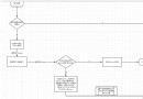
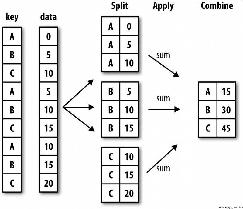
Hadley Wickham( Many popular R Author of the language pack ) Created a term for grouping operations "split-apply-combine"( Split - application - Merge ). First stage ,pandas object ( Whether it's Series、DataFrame Or something else ) The data in will be split according to one or more keys you provide (split) For multiple groups . The split operation is performed on a specific axis of the object . for example ,DataFrame Can be in its line (axis=0) Or column (axis=1) Group on . then , Apply a function to (apply) To each group and generate a new value . Last , The execution results of all these functions are merged (combine) To the final result object . The form of the result object generally depends on the operations performed on the data . chart 10-1 A simple grouping aggregation process is roughly described .
Grouping keys can take many forms , And the types don't have to be the same :
Be careful , The last three are just shortcuts , The ultimate goal is still to produce a set of values for splitting objects . If you think these things look very abstract , Never mind , I'll give you a lot of examples of this in this chapter . First, let's take a look at this very simple tabular data set ( With DataFrame In the form of ):
In [10]: df = pd.DataFrame({
'key1' : ['a', 'a', 'b', 'b', 'a'],
....: 'key2' : ['one', 'two', 'one', 'two', 'one'],
....: 'data1' : np.random.randn(5),
....: 'data2' : np.random.randn(5)})
In [11]: df
Out[11]:
data1 data2 key1 key2
0 -0.204708 1.393406 a one
1 0.478943 0.092908 a two
2 -0.519439 0.281746 b one
3 -0.555730 0.769023 b two
4 1.965781 1.246435 a one
Suppose you want to press key1 Grouping , And calculate data1 The average of the columns . There are many ways to implement this function , What we need here is : visit data1, And according to key1 call groupby:
In [12]: grouped = df['data1'].groupby(df['key1'])
In [13]: grouped
Out[13]: <pandas.core.groupby.SeriesGroupBy object at 0x7faa31537390>
Variable grouped It's a GroupBy object . It hasn't actually done any calculations yet , It just contains some grouping keys df[‘key1’] Just intermediate data . let me put it another way , The object already has all the information it needs to perform the next operation on each group . for example , We can call GroupBy Of mean Method to calculate the group average :
In [14]: grouped.mean()
Out[14]:
key1
a 0.746672
b -0.537585
Name: data1, dtype: float64
I will explain in detail later .mean() Call procedure for . The most important thing here , data (Series) Aggregation is carried out according to the grouping key , A new Series, Its index is key1 Unique value in column . The reason why the name of the index in the result is key1, Because of the primitive DataFrame The column of df[‘key1’] That's the name .
If we pass in a list of multiple arrays at once , You get different results :
In [15]: means = df['data1'].groupby([df['key1'], df['key2']]).mean()
In [16]: means
Out[16]:
key1 key2
a one 0.880536
two 0.478943
b one -0.519439
two -0.555730
Name: data1, dtype: float64
here , I grouped the data with two keys , Got Series With a hierarchical index ( Consisting of unique key pairs ):
In [17]: means.unstack()
Out[17]:
key2 one two
key1
a 0.880536 0.478943
b -0.519439 -0.555730
In this case , The grouping keys are Series. actually , The grouping key can be any array of appropriate length :
In [18]: states = np.array(['Ohio', 'California', 'California', 'Ohio', 'Ohio'])
In [19]: years = np.array([2005, 2005, 2006, 2005, 2006])
In [20]: df['data1'].groupby([states, years]).mean()
Out[20]:
California 2005 0.478943
2006 -0.519439
Ohio 2005 -0.380219
2006 1.965781
Name: data1, dtype: float64
Usually , The grouping information is in the same place to be processed DataFrame in . here , You can also list ( Can be a string 、 Numbers or other Python object ) Used as grouping key :
In [21]: df.groupby('key1').mean()
Out[21]:
data1 data2
key1
a 0.746672 0.910916
b -0.537585 0.525384
In [22]: df.groupby(['key1', 'key2']).mean()
Out[22]:
data1 data2
key1 key2
a one 0.880536 1.319920
two 0.478943 0.092908
b one -0.519439 0.281746
two -0.555730 0.769023
You may have noticed , The first example is executing df.groupby(‘key1’).mean() when , There is no key2 Column . This is because df[‘key2’] Not numerical data ( Be commonly called “ Trouble column ”), So it was excluded from the results . By default , All numeric columns are aggregated , Although sometimes it may be filtered into a subset , I'll meet you later .
Whether you are ready to take groupby What do you do , May be used GroupBy Of size Method , It can return a with the size of the group Series:
In [23]: df.groupby(['key1', 'key2']).size()
Out[23]:
key1 key2
a one 2
two 1
b one 1
two 1
dtype: int64
Be careful , Missing values in any grouping keyword , Will be removed from the results .
GroupBy Object supports iteration , Can produce a set of binary groups ( It consists of group name and data block ). See the following example :
In [24]: for name, group in df.groupby('key1'):
....: print(name)
....: print(group)
....:
a
data1 data2 key1 key2
0 -0.204708 1.393406 a one
1 0.478943 0.092908 a two
4 1.965781 1.246435 a one
b
data1 data2 key1 key2
2 -0.519439 0.281746 b one
3 -0.555730 0.769023 b two
In the case of multiple bonds , The first element of a tuple will be a tuple of key values :
In [25]: for (k1, k2), group in df.groupby(['key1', 'key2']):
....: print((k1, k2))
....: print(group)
....:
('a', 'one')
data1 data2 key1 key2
0 -0.204708 1.393406 a one
4 1.965781 1.246435 a one
('a', 'two')
data1 data2 key1 key2
1 0.478943 0.092908 a two
('b', 'one')
data1 data2 key1 key2
2 -0.519439 0.281746 b one
('b', 'two')
data1 data2 key1 key2
3 -0.55573 0.769023 b two
Of course , You can do anything with these pieces of data . There is an operation that you may find useful : Make these data fragments into a dictionary :
In [26]: pieces = dict(list(df.groupby('key1')))
In [27]: pieces['b']
Out[27]:
data1 data2 key1 key2
2 -0.519439 0.281746 b one
3 -0.555730 0.769023 b two
groupby The default is in axis=0 Grouped on , You can also group on any other axis by setting . Take the example above df Come on , We can use dtype Group Columns :
In [28]: df.dtypes
Out[28]:
data1 float64
data2 float64
key1 object
key2 object
dtype: object
In [29]: grouped = df.groupby(df.dtypes, axis=1)
You can print groups as follows :
In [30]: for dtype, group in grouped:
....: print(dtype)
....: print(group)
....:
float64
data1 data2
0 -0.204708 1.393406
1 0.478943 0.092908
2 -0.519439 0.281746
3 -0.555730 0.769023
4 1.965781 1.246435
object
key1 key2
0 a one
1 a two
2 b one
3 b two
4 a one
For the DataFrame Produced GroupBy object , If you use one ( Single string ) Or a group ( Array of strings ) Column name to index it , You can select some columns for aggregation . in other words :
df.groupby('key1')['data1']
df.groupby('key1')[['data2']]
Is the syntax sugar of the following code :
df['data1'].groupby(df['key1'])
df[['data2']].groupby(df['key1'])
Especially for big data sets , Most likely, you only need to aggregate some columns . for example , In the previous dataset , If you only need to calculate data2 The average value of the column and in DataFrame Form the result , It can be written like this :
In [31]: df.groupby(['key1', 'key2'])[['data2']].mean()
Out[31]:
data2
key1 key2
a one 1.319920
two 0.092908
b one 0.281746
two 0.769023
The object returned by this index operation is a grouped DataFrame( If you pass in a list or array ) Or grouped Series( If you pass in a single column name in scalar form ):
In [32]: s_grouped = df.groupby(['key1', 'key2'])['data2']
In [33]: s_grouped
Out[33]: <pandas.core.groupby.SeriesGroupBy object at 0x7faa30c78da0>
In [34]: s_grouped.mean()
Out[34]:
key1 key2
a one 1.319920
two 0.092908
b one 0.281746
two 0.769023
Name: data2, dtype: float64
## Through a dictionary or Series Grouping
Except for arrays , The grouping information can also exist in other forms . Let's look at another example DataFrame:
In [35]: people = pd.DataFrame(np.random.randn(5, 5),
....: columns=['a', 'b', 'c', 'd', 'e'],
....: index=['Joe', 'Steve', 'Wes', 'Jim', 'Travis'])
In [36]: people.iloc[2:3, [1, 2]] = np.nan # Add a few NA values
In [37]: people
Out[37]:
a b c d e
Joe 1.007189 -1.296221 0.274992 0.228913 1.352917
Steve 0.886429 -2.001637 -0.371843 1.669025 -0.438570
Wes -0.539741 NaN NaN -1.021228 -0.577087
Jim 0.124121 0.302614 0.523772 0.000940 1.343810
Travis -0.713544 -0.831154 -2.370232 -1.860761 -0.860757
Now? , Suppose you know the grouping relationship of the columns , And you want to calculate the sum of columns according to the grouping :
In [38]: mapping = {
'a': 'red', 'b': 'red', 'c': 'blue',
....: 'd': 'blue', 'e': 'red', 'f' : 'orange'}
Now? , You can pass this dictionary on to groupby, To construct an array , But we can pass the dictionary directly ( I included the key “f” To emphasize , It is possible to have unused grouping keys ):
In [39]: by_column = people.groupby(mapping, axis=1)
In [40]: by_column.sum()
Out[40]:
blue red
Joe 0.503905 1.063885
Steve 1.297183 -1.553778
Wes -1.021228 -1.116829
Jim 0.524712 1.770545
Travis -4.230992 -2.405455
Series It has the same function , It can be thought of as a fixed size mapping :
In [41]: map_series = pd.Series(mapping)
In [42]: map_series
Out[42]:
a red
b red
c blue
d blue
e red
f orange
dtype: object
In [43]: people.groupby(map_series, axis=1).count()
Out[43]:
blue red
Joe 2 3
Steve 2 3
Wes 1 2
Jim 2 3
Travis 2 3
## Grouping by function
Rather than using a dictionary or Series, Use Python Function is a more native way to define group mappings . Any function that is treated as a grouping key will be called once on each index value , Its return value will be used as the group name . Specifically speaking , The example in the previous section DataFrame For example , The index value is the name of the person . You can calculate an array of string lengths , A simpler way is to pass in len function :
In [44]: people.groupby(len).sum()
Out[44]:
a b c d e
3 0.591569 -0.993608 0.798764 -0.791374 2.119639
5 0.886429 -2.001637 -0.371843 1.669025 -0.438570
6 -0.713544 -0.831154 -2.370232 -1.860761 -0.860757
Follow the function with the array 、 list 、 Dictionaries 、Series Mixing is not a problem , Because everything is internally converted to an array :
In [45]: key_list = ['one', 'one', 'one', 'two', 'two']
In [46]: people.groupby([len, key_list]).min()
Out[46]:
a b c d e
3 one -0.539741 -1.296221 0.274992 -1.021228 -0.577087
two 0.124121 0.302614 0.523772 0.000940 1.343810
5 one 0.886429 -2.001637 -0.371843 1.669025 -0.438570
6 two -0.713544 -0.831154 -2.370232 -1.860761 -0.860757
The most convenient place for a hierarchical index dataset is that it can aggregate according to one level of the axis index :
In [47]: columns = pd.MultiIndex.from_arrays([['US', 'US', 'US', 'JP', 'JP'],
....: [1, 3, 5, 1, 3]],
....: names=['cty', 'tenor'])
In [48]: hier_df = pd.DataFrame(np.random.randn(4, 5), columns=columns)
In [49]: hier_df
Out[49]:
cty US JP
tenor 1 3 5 1 3
0 0.560145 -1.265934 0.119827 -1.063512 0.332883
1 -2.359419 -0.199543 -1.541996 -0.970736 -1.307030
2 0.286350 0.377984 -0.753887 0.331286 1.349742
3 0.069877 0.246674 -0.011862 1.004812 1.327195
To group by level , Use level Keyword pass level sequence number or name :
In [50]: hier_df.groupby(level='cty', axis=1).count()
Out[50]:
cty JP US
0 2 3
1 2 3
2 2 3
3 2 3
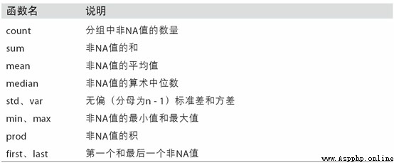
Aggregation refers to any data conversion process that generates scalar values from an array . Some of the previous examples have been used , such as mean、count、min as well as sum etc. . You may want to know where GroupBy Object mean() What happened when . Many common aggregation operations ( As shown in the table 10-1 Shown ) Have been optimized . However , In addition to these methods , You can also use other .
You can use your own aggregation algorithm , You can also call any method already defined on the grouped object . for example ,quantile You can calculate Series or DataFrame Sample quantile of column .
although quantile Not explicitly implemented in GroupBy, But it's a Series Method , So here's what works . actually ,GroupBy Will be effective in Series Slice , Then call... For each slice piece.quantile(0.9), Finally, these results are assembled into the final results :
In [51]: df
Out[51]:
data1 data2 key1 key2
0 -0.204708 1.393406 a one
1 0.478943 0.092908 a two
2 -0.519439 0.281746 b one
3 -0.555730 0.769023 b two
4 1.965781 1.246435 a one
In [52]: grouped = df.groupby('key1')
In [53]: grouped['data1'].quantile(0.9)
Out[53]:
key1
a 1.668413
b -0.523068
Name: data1, dtype: float64
If you want to use your own aggregate function , Just pass it in aggregate or agg The method can :
In [54]: def peak_to_peak(arr):
....: return arr.max() - arr.min()
In [55]: grouped.agg(peak_to_peak)
Out[55]:
data1 data2
key1
a 2.170488 1.300498
b 0.036292 0.487276
You may have noticed , Some ways ( Such as describe) It can also be used here , Even strictly speaking , They are not aggregation operations :
In [56]: grouped.describe()
Out[56]:
data1 \
count mean std min 25% 50% 75%
key1
a 3.0 0.746672 1.109736 -0.204708 0.137118 0.478943 1.222362
b 2.0 -0.537585 0.025662 -0.555730 -0.546657 -0.537585 -0.528512
data2 \
max count mean std min 25% 50%
key1
a 1.965781 3.0 0.910916 0.712217 0.092908 0.669671 1.246435
b -0.519439 2.0 0.525384 0.344556 0.281746 0.403565 0.525384
75% max
key1
a 1.319920 1.393406
b 0.647203 0.769023
In the rear 10.3 section , I will elaborate on what this is all about .
note : Custom aggregate functions are better than tables 10-1 The optimized functions in are much slower . This is because there is a very large overhead in constructing intermediate packet data blocks ( Function call 、 Data rearrangement, etc ).
Back to the previous tip example . Use read_csv After importing data , We added a column for the tip percentage tip_pct:
In [57]: tips = pd.read_csv('examples/tips.csv')
# Add tip percentage of total bill
In [58]: tips['tip_pct'] = tips['tip'] / tips['total_bill']
In [59]: tips[:6]
Out[59]:
total_bill tip smoker day time size tip_pct
0 16.99 1.01 No Sun Dinner 2 0.059447
1 10.34 1.66 No Sun Dinner 3 0.160542
2 21.01 3.50 No Sun Dinner 3 0.166587
3 23.68 3.31 No Sun Dinner 2 0.139780
4 24.59 3.61 No Sun Dinner 4 0.146808
5 25.29 4.71 No Sun Dinner 4 0.186240
You've seen , Yes Series or DataFrame The column aggregation operation actually uses aggregate( Use custom functions ) Or call something like mean、std Something like that . However , You may want to use different aggregate functions for different columns , Or apply multiple functions at once . In fact, it's easy to do , I will use some examples to explain . First , According to heaven and smoker Yes tips Grouping :
In [60]: grouped = tips.groupby(['day', 'smoker'])
Be careful , For tables 10-1 The descriptive statistics in , You can pass the function name as a string :
In [61]: grouped_pct = grouped['tip_pct']
In [62]: grouped_pct.agg('mean')
Out[62]:
day smoker
Fri No 0.151650
Yes 0.174783
Sat No 0.158048
Yes 0.147906
Sun No 0.160113
Yes 0.187250
Thur No 0.160298
Yes 0.163863
Name: tip_pct, dtype: float64
If you pass in a set of functions or function names , Got DataFrame The column of will be named after the corresponding function :
In [63]: grouped_pct.agg(['mean', 'std', peak_to_peak])
Out[63]:
mean std peak_to_peak
day smoker
Fri No 0.151650 0.028123 0.067349
Yes 0.174783 0.051293 0.159925
Sat No 0.158048 0.039767 0.235193
Yes 0.147906 0.061375 0.290095
Sun No 0.160113 0.042347 0.193226
Yes 0.187250 0.154134 0.644685
Thur No 0.160298 0.038774 0.193350
Yes 0.163863 0.039389 0.151240
here , We passed a set of aggregate functions to aggregate , Evaluate data groups independently .
You don't have to accept GroupBy Those column names given automatically , especially lambda function , Their names are ’', Such recognition is very low ( Through function __name__ Just look at the properties ). therefore , If the incoming one is from (name,function) A list of tuples , Then the first element of each tuple will be used as DataFrame Column name of ( You can think of this list of binary tuples as an ordered map ):
In [64]: grouped_pct.agg([('foo', 'mean'), ('bar', np.std)])
Out[64]:
foo bar
day smoker
Fri No 0.151650 0.028123
Yes 0.174783 0.051293
Sat No 0.158048 0.039767
Yes 0.147906 0.061375
Sun No 0.160113 0.042347
Yes 0.187250 0.154134
Thur No 0.160298 0.038774
Yes 0.163863 0.039389
about DataFrame, You have more options , You can define a set of functions that apply to all columns , Or different columns apply different functions . Suppose we want to be right tip_pct and total_bill Column calculates three statistics :
In [65]: functions = ['count', 'mean', 'max']
In [66]: result = grouped['tip_pct', 'total_bill'].agg(functions)
In [67]: result
Out[67]:
tip_pct total_bill
count mean max count mean max
day smoker
Fri No 4 0.151650 0.187735 4 18.420000 22.75
Yes 15 0.174783 0.263480 15 16.813333 40.17
Sat No 45 0.158048 0.291990 45 19.661778 48.33
Yes 42 0.147906 0.325733 42 21.276667 50.81
Sun No 57 0.160113 0.252672 57 20.506667 48.17
Yes 19 0.187250 0.710345 19 24.120000 45.35
Thur No 45 0.160298 0.266312 45 17.113111 41.19
Yes 17 0.163863 0.241255 17 19.190588 43.11
As you can see , result DataFrame Have hierarchical Columns , This is equivalent to aggregating the columns separately , And then use concat Put the results together , Use column names as keys Parameters :
In [68]: result['tip_pct']
Out[68]:
count mean max
day smoker
Fri No 4 0.151650 0.187735
Yes 15 0.174783 0.263480
Sat No 45 0.158048 0.291990
Yes 42 0.147906 0.325733
Sun No 57 0.160113 0.252672
Yes 19 0.187250 0.710345
Thur No 45 0.160298 0.266312
Yes 17 0.163863 0.241255
It's the same as before , You can also pass in a set of tuples with custom names :
In [69]: ftuples = [('Durchschnitt', 'mean'),('Abweichung', np.var)]
In [70]: grouped['tip_pct', 'total_bill'].agg(ftuples)
Out[70]:
tip_pct total_bill
Durchschnitt Abweichung Durchschnitt Abweichung
day smoker
Fri No 0.151650 0.000791 18.420000 25.596333
Yes 0.174783 0.002631 16.813333 82.562438
Sat No 0.158048 0.001581 19.661778 79.908965
Yes 0.147906 0.003767 21.276667 101.387535
Sun No 0.160113 0.001793 20.506667 66.099980
Yes 0.187250 0.023757 24.120000 109.046044
Thur No 0.160298 0.001503 17.113111 59.625081
Yes 0.163863 0.001551 19.190588 69.808518
Now? , Suppose you want to apply different functions to a column or to different columns . The specific method is to agg Pass in a dictionary that maps column names to functions :
In [71]: grouped.agg({
'tip' : np.max, 'size' : 'sum'})
Out[71]:
tip size
day smoker
Fri No 3.50 9
Yes 4.73 31
Sat No 9.00 115
Yes 10.00 104
Sun No 6.00 167
Yes 6.50 49
Thur No 6.70 112
Yes 5.00 40
In [72]: grouped.agg({
'tip_pct' : ['min', 'max', 'mean', 'std'],
....: 'size' : 'sum'})
Out[72]:
tip_pct size
min max mean std sum
day smoker
Fri No 0.120385 0.187735 0.151650 0.028123 9
Yes 0.103555 0.263480 0.174783 0.051293 31
Sat No 0.056797 0.291990 0.158048 0.039767 115
Yes 0.035638 0.325733 0.147906 0.061375 104
Sun No 0.059447 0.252672 0.160113 0.042347 167
Yes 0.065660 0.710345 0.187250 0.154134 49
Thur No 0.072961 0.266312 0.160298 0.038774 112
Yes 0.090014 0.241255 0.163863 0.039389 40
Only when multiple functions are applied to at least one column ,DataFrame Will have hierarchical Columns .
up to now , The aggregated data in all examples has an index consisting of unique grouping keys ( It may be hierarchical ). Because it is not always necessary , So you can ask groupby Pass in as_index=False To disable this feature :
In [73]: tips.groupby(['day', 'smoker'], as_index=False).mean()
Out[73]:
day smoker total_bill tip size tip_pct
0 Fri No 18.420000 2.812500 2.250000 0.151650
1 Fri Yes 16.813333 2.714000 2.066667 0.174783
2 Sat No 19.661778 3.102889 2.555556 0.158048
3 Sat Yes 21.276667 2.875476 2.476190 0.147906
4 Sun No 20.506667 3.167895 2.929825 0.160113
5 Sun Yes 24.120000 3.516842 2.578947 0.187250
6 Thur No 17.113111 2.673778 2.488889 0.160298
7 Thur Yes 19.190588 3.030000 2.352941 0.163863
Of course , Call... On the result reset_index You can also get results in this form . Use as_index=False Method can avoid some unnecessary calculations .
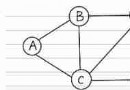
Most versatile GroupBy The method is apply, The rest of this section will focus on it . Pictured 10-2 Shown ,apply The object to be processed will be split into multiple fragments , Then call the incoming function on each fragment , Finally, try to put the pieces together .
Back to the previous tip data set , Suppose you want to choose the highest one according to the group 5 individual tip_pct value . First , Write a function to select the row with the maximum value in the specified column :
In [74]: def top(df, n=5, column='tip_pct'):
....: return df.sort_values(by=column)[-n:]
In [75]: top(tips, n=6)
Out[75]:
total_bill tip smoker day time size tip_pct
109 14.31 4.00 Yes Sat Dinner 2 0.279525
183 23.17 6.50 Yes Sun Dinner 4 0.280535
232 11.61 3.39 No Sat Dinner 2 0.291990
67 3.07 1.00 Yes Sat Dinner 1 0.325733
178 9.60 4.00 Yes Sun Dinner 2 0.416667
172 7.25 5.15 Yes Sun Dinner 2 0.710345
Now? , If the smoker Group and call... With this function apply, Will get :
In [76]: tips.groupby('smoker').apply(top)
Out[76]:
total_bill tip smoker day time size tip_pct
smoker
No 88 24.71 5.85 No Thur Lunch 2 0.236746
185 20.69 5.00 No Sun Dinner 5 0.241663
51 10.29 2.60 No Sun Dinner 2 0.252672
149 7.51 2.00 No Thur Lunch 2 0.266312
232 11.61 3.39 No Sat Dinner 2 0.291990
Yes 109 14.31 4.00 Yes Sat Dinner 2 0.279525
183 23.17 6.50 Yes Sun Dinner 4 0.280535
67 3.07 1.00 Yes Sat Dinner 1 0.325733
178 9.60 4.00 Yes Sun Dinner 2 0.416667
172 7.25 5.15 Yes Sun Dinner 2 0.710345
What happened here ?top Function in DataFrame Called on each fragment of , Then the result is pandas.concat Put it together , And marked with the group name . therefore , The end result is a hierarchical index , The inner index value comes from the original DataFrame.
If to apply Functions that accept other parameters or keywords , These contents can be passed in after the function name :
In [77]: tips.groupby(['smoker', 'day']).apply(top, n=1, column='total_bill')
Out[77]:
total_bill tip smoker day time size tip_pct
smoker day
No Fri 94 22.75 3.25 No Fri Dinner 2 0.142857
Sat 212 48.33 9.00 No Sat Dinner 4 0.186220
Sun 156 48.17 5.00 No Sun Dinner 6 0.103799
Thur 142 41.19 5.00 No Thur Lunch 5 0.121389
Yes Fri 95 40.17 4.73 Yes Fri Dinner 4 0.117750
Sat 170 50.81 10.00 Yes Sat Dinner 3 0.196812
Sun 182 45.35 3.50 Yes Sun Dinner 3 0.077178
Thur 197 43.11 5.00 Yes Thur Lunch 4 0.115982
note : In addition to these basic uses , Can you give full play to apply The power of depends largely on your creativity . What the incoming function can do is up to you to decide , It just needs to return one pandas Object or scalar value . The examples in subsequent parts of this chapter are mainly used to explain how to use groupby Solve all kinds of problems .
Maybe you already remember , I was in GroupBy Object called describe:
In [78]: result = tips.groupby('smoker')['tip_pct'].describe()
In [79]: result
Out[79]:
count mean std min 25% 50% 75% \
smoker
No 151.0 0.159328 0.039910 0.056797 0.136906 0.155625 0.185014
Yes 93.0 0.163196 0.085119 0.035638 0.106771 0.153846 0.195059
max
smoker
No 0.291990
Yes 0.710345
In [80]: result.unstack('smoker')
Out[80]:
smoker
count No 151.000000
Yes 93.000000
mean No 0.159328
Yes 0.163196
std No 0.039910
Yes 0.085119
min No 0.056797
Yes 0.035638
25% No 0.136906
Yes 0.106771
50% No 0.155625
Yes 0.153846
75% No 0.185014
Yes 0.195059
max No 0.291990
Yes 0.710345
dtype: float64
stay GroupBy in , When you call something like describe And so on , In fact, it's just a shortcut that applies the following two codes :
f = lambda x: x.describe()
grouped.apply(f)
As you can see from the example above , The grouping key, together with the index of the original object, constitutes a hierarchical index in the result object . take group_keys=False Pass in groupby To disable the effect :
In [81]: tips.groupby('smoker', group_keys=False).apply(top)
Out[81]:
total_bill tip smoker day time size tip_pct
88 24.71 5.85 No Thur Lunch 2 0.236746
185 20.69 5.00 No Sun Dinner 5 0.241663
51 10.29 2.60 No Sun Dinner 2 0.252672
149 7.51 2.00 No Thur Lunch 2 0.266312
232 11.61 3.39 No Sat Dinner 2 0.291990
109 14.31 4.00 Yes Sat Dinner 2 0.279525
183 23.17 6.50 Yes Sun Dinner 4 0.280535
67 3.07 1.00 Yes Sat Dinner 1 0.325733
178 9.60 4.00 Yes Sun Dinner 2 0.416667
172 7.25 5.15 Yes Sun Dinner 2 0.710345
I was in the 8 It's mentioned in the chapter ,pandas There are some tools that can split data into multiple blocks according to the specified bin or sample quantile ( such as cut and qcut). Follow these functions with groupby Combine , It is very easy to implement the bucket of data set (bucket) Or quantile (quantile) Analysis of the . Take the following simple random data set as an example , We make use of cut Put them in barrels of equal length :
In [82]: frame = pd.DataFrame({
'data1': np.random.randn(1000),
....: 'data2': np.random.randn(1000)})
In [83]: quartiles = pd.cut(frame.data1, 4)
In [84]: quartiles[:10]
Out[84]:
0 (-1.23, 0.489]
1 (-2.956, -1.23]
2 (-1.23, 0.489]
3 (0.489, 2.208]
4 (-1.23, 0.489]
5 (0.489, 2.208]
6 (-1.23, 0.489]
7 (-1.23, 0.489]
8 (0.489, 2.208]
9 (0.489, 2.208]
Name: data1, dtype: category
Categories (4, interval[float64]): [(-2.956, -1.23] < (-1.23, 0.489] < (0.489, 2.
208] < (2.208, 3.928]]
from cut Back to Categorical Objects can be passed directly to groupby. therefore , We can do it like this data2 Column to do some statistical calculations :
In [85]: def get_stats(group):
....: return {
'min': group.min(), 'max': group.max(),
....: 'count': group.count(), 'mean': group.mean()}
In [86]: grouped = frame.data2.groupby(quartiles)
In [87]: grouped.apply(get_stats).unstack()
Out[87]:
count max mean min
data1
(-2.956, -1.23] 95.0 1.670835 -0.039521 -3.399312
(-1.23, 0.489] 598.0 3.260383 -0.002051 -2.989741
(0.489, 2.208] 297.0 2.954439 0.081822 -3.745356
(2.208, 3.928] 10.0 1.765640 0.024750 -1.929776
These are barrels of equal length . To get barrels of equal size according to the sample quantile , Use qcut that will do . Pass in labels=False Only quantile numbers can be obtained :
# Return quantile numbers
In [88]: grouping = pd.qcut(frame.data1, 10, labels=False)
In [89]: grouped = frame.data2.groupby(grouping)
In [90]: grouped.apply(get_stats).unstack()
Out[90]:
count max mean min
data1
0 100.0 1.670835 -0.049902 -3.399312
1 100.0 2.628441 0.030989 -1.950098
2 100.0 2.527939 -0.067179 -2.925113
3 100.0 3.260383 0.065713 -2.315555
4 100.0 2.074345 -0.111653 -2.047939
5 100.0 2.184810 0.052130 -2.989741
6 100.0 2.458842 -0.021489 -2.223506
7 100.0 2.954439 -0.026459 -3.056990
8 100.0 2.735527 0.103406 -3.745356
9 100.0 2.377020 0.220122 -2.064111
We will be in the 12 This chapter explains in detail pandas Of Categorical type .
Clean up the missing data , Sometimes you use dropna Replace it with , Sometimes you may want to fill in with a fixed value or a value derived from the dataset itself NA value . You have to use fillna This tool . In the following example , I use the average to fill in NA value :
In [91]: s = pd.Series(np.random.randn(6))
In [92]: s[::2] = np.nan
In [93]: s
Out[93]:
0 NaN
1 -0.125921
2 NaN
3 -0.884475
4 NaN
5 0.227290
dtype: float64
In [94]: s.fillna(s.mean())
Out[94]:
0 -0.261035
1 -0.125921
2 -0.261035
3 -0.884475
4 -0.261035
5 0.227290
dtype: float64
Suppose you need to fill in different values for different groups . One way is to group data , And use apply And one that can call on each data block fillna The function of . Here are some sample data about several states in the United States , These states are divided into the East and the West :
In [95]: states = ['Ohio', 'New York', 'Vermont', 'Florida',
....: 'Oregon', 'Nevada', 'California', 'Idaho']
In [96]: group_key = ['East'] * 4 + ['West'] * 4
In [97]: data = pd.Series(np.random.randn(8), index=states)
In [98]: data
Out[98]:
Ohio 0.922264
New York -2.153545
Vermont -0.365757
Florida -0.375842
Oregon 0.329939
Nevada 0.981994
California 1.105913
Idaho -1.613716
dtype: float64
[‘East’] * 4 Produces a list , It includes [‘East’] Four copies of elements in . Concatenate these lists .
Set some values as missing :
In [99]: data[['Vermont', 'Nevada', 'Idaho']] = np.nan
In [100]: data
Out[100]:
Ohio 0.922264
New York -2.153545
Vermont NaN
Florida -0.375842
Oregon 0.329939
Nevada NaN
California 1.105913
Idaho NaN
dtype: float64
In [101]: data.groupby(group_key).mean()
Out[101]:
East -0.535707
West 0.717926
dtype: float64
We can use the group average to fill NA value :
In [102]: fill_mean = lambda g: g.fillna(g.mean())
In [103]: data.groupby(group_key).apply(fill_mean)
Out[103]:
Ohio 0.922264
New York -2.153545
Vermont -0.535707
Florida -0.375842
Oregon 0.329939
Nevada 0.717926
California 1.105913
Idaho 0.717926
dtype: float64
in addition , You can also predefine the fill values for each group in your code . Because the group has a name attribute , So we can use it :
In [104]: fill_values = {
'East': 0.5, 'West': -1}
In [105]: fill_func = lambda g: g.fillna(fill_values[g.name])
In [106]: data.groupby(group_key).apply(fill_func)
Out[106]:
Ohio 0.922264
New York -2.153545
Vermont 0.500000
Florida -0.375842
Oregon 0.329939
Nevada -1.000000
California 1.105913
Idaho -1.000000
dtype: float64
Suppose you want to randomly select from a large data set ( To replace or not to replace ) Samples for Monte Carlo simulation (Monte Carlo simulation) Or other analytical work .“ extract ” There are many ways , The method used here is right Series Use sample Method :
# Hearts, Spades, Clubs, Diamonds
suits = ['H', 'S', 'C', 'D']
card_val = (list(range(1, 11)) + [10] * 3) * 4
base_names = ['A'] + list(range(2, 11)) + ['J', 'K', 'Q']
cards = []
for suit in ['H', 'S', 'C', 'D']:
cards.extend(str(num) + suit for num in base_names)
deck = pd.Series(card_val, index=cards)
Now I have a length of 52 Of Series, The index includes the brand name , The value is 21 Points or points used for scoring in other games ( For the sake of simplicity , I should A The number of points is 1):
In [108]: deck[:13]
Out[108]:
AH 1
2H 2
3H 3
4H 4
5H 5
6H 6
7H 7
8H 8
9H 9
10H 10
JH 10
KH 10
QH 10
dtype: int64
Now? , According to what I said above , Draw from the deck 5 Zhang , The code is as follows :
In [109]: def draw(deck, n=5):
.....: return deck.sample(n)
In [110]: draw(deck)
Out[110]:
AD 1
8C 8
5H 5
KC 10
2C 2
dtype: int64
Suppose you want to draw two cards at random from each suit . Because the suit is the last character of the card name , So we can group according to this , And use apply:
In [111]: get_suit = lambda card: card[-1] # last letter is suit
In [112]: deck.groupby(get_suit).apply(draw, n=2)
Out[112]:
C 2C 2
3C 3
D KD 10
8D 8
H KH 10
3H 3
S 2S 2
4S 4
dtype: int64
perhaps , You can also write like this :
In [113]: deck.groupby(get_suit, group_keys=False).apply(draw, n=2)
Out[113]:
KC 10
JC 10
AD 1
5D 5
5H 5
6H 6
7S 7
KS 10
dtype: int64
according to groupby Of “ Split - application - Merge ” normal form , Can be done DataFrame Between columns or between two Series Operation between ( For example, group weighted average ). Take the following data set as an example , It contains grouping keys 、 Value and some weight values :
In [114]: df = pd.DataFrame({
'category': ['a', 'a', 'a', 'a',
.....: 'b', 'b', 'b', 'b'],
.....: 'data': np.random.randn(8),
.....: 'weights': np.random.rand(8)})
In [115]: df
Out[115]:
category data weights
0 a 1.561587 0.957515
1 a 1.219984 0.347267
2 a -0.482239 0.581362
3 a 0.315667 0.217091
4 b -0.047852 0.894406
5 b -0.454145 0.918564
6 b -0.556774 0.277825
7 b 0.253321 0.955905
Then you can use category Calculate the group weighted average :
In [116]: grouped = df.groupby('category')
In [117]: get_wavg = lambda g: np.average(g['data'], weights=g['weights'])
In [118]: grouped.apply(get_wavg)
Out[118]:
category
a 0.811643
b -0.122262
dtype: float64
Another example , Consider a question from Yahoo!Finance Data set of , It contains several stocks and standard & Poor's 500 Index ( Symbol SPX) The closing price of :
In [119]: close_px = pd.read_csv('examples/stock_px_2.csv', parse_dates=True,
.....: index_col=0)
In [120]: close_px.info()
<class 'pandas.core.frame.DataFrame'>
DatetimeIndex: 2214 entries, 2003-01-02 to 2011-10-14
Data columns (total 4 columns):
AAPL 2214 non-null float64
MSFT 2214 non-null float64
XOM 2214 non-null float64
SPX 2214 non-null float64
dtypes: float64(4)
memory usage: 86.5 KB
In [121]: close_px[-4:]
Out[121]:
AAPL MSFT XOM SPX
2011-10-11 400.29 27.00 76.27 1195.54
2011-10-12 402.19 26.96 77.16 1207.25
2011-10-13 408.43 27.18 76.37 1203.66
2011-10-14 422.00 27.27 78.11 1224.58
To do a more interesting task : Calculate a daily rate of return ( Calculate by percentage change ) And SPX The annual correlation coefficient between DataFrame. Here is an implementation , Let's first create a function , Use it to calculate the sum of each column SPX Pairwise correlation coefficient of columns :
In [122]: spx_corr = lambda x: x.corrwith(x['SPX'])
Next , We use pct_change Calculation close_px Percent change in :
In [123]: rets = close_px.pct_change().dropna()
Last , We grouped the percentage changes by year , You can use a one line function , Returns each... From the label of each row datetime Labeled year attribute :
In [124]: get_year = lambda x: x.year
In [125]: by_year = rets.groupby(get_year)
In [126]: by_year.apply(spx_corr)
Out[126]:
AAPL MSFT XOM SPX
2003 0.541124 0.745174 0.661265 1.0
2004 0.374283 0.588531 0.557742 1.0
2005 0.467540 0.562374 0.631010 1.0
2006 0.428267 0.406126 0.518514 1.0
2007 0.508118 0.658770 0.786264 1.0
2008 0.681434 0.804626 0.828303 1.0
2009 0.707103 0.654902 0.797921 1.0
2010 0.710105 0.730118 0.839057 1.0
2011 0.691931 0.800996 0.859975 1.0
Of course , You can also calculate the correlation coefficient between columns . here , We calculated Apple and Microsoft Annual correlation coefficient of :
In [127]: by_year.apply(lambda g: g['AAPL'].corr(g['MSFT']))
Out[127]:
2003 0.480868
2004 0.259024
2005 0.300093
2006 0.161735
2007 0.417738
2008 0.611901
2009 0.432738
2010 0.571946
2011 0.581987
dtype: float64
Continue with the previous example , You can use it. groupby Perform more complex group statistical analysis , As long as the function returns pandas Object or scalar value . for example , I can define the following regress function ( utilize statsmodels Econometrics library ) Perform ordinary least squares on each data block (Ordinary Least Squares,OLS) Return to :
import statsmodels.api as sm
def regress(data, yvar, xvars):
Y = data[yvar]
X = data[xvars]
X['intercept'] = 1.
result = sm.OLS(Y, X).fit()
return result.params
Now? , In order to calculate by year AAPL Yes SPX Linear regression of yield , perform :
In [129]: by_year.apply(regress, 'AAPL', ['SPX'])
Out[129]:
SPX intercept
2003 1.195406 0.000710
2004 1.363463 0.004201
2005 1.766415 0.003246
2006 1.645496 0.000080
2007 1.198761 0.003438
2008 0.968016 -0.001110
2009 0.879103 0.002954
2010 1.052608 0.001261
2011 0.806605 0.001514
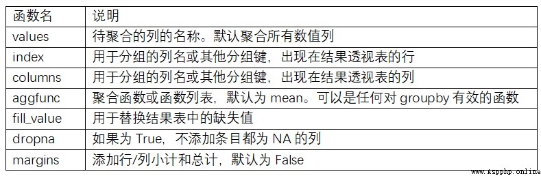
PivotTable (pivot table) It is a common data summary tool in various spreadsheet programs and other data analysis software . It aggregates data based on one or more keys , And according to the grouping key on the row and column, the data is allocated to each rectangular area . stay Python and pandas in , You can use the groupby Functions and ( Capable of utilizing hierarchical indexes ) Reshape operation to make pivot table .DataFrame There is one pivot_table Method , There is also a top class pandas.pivot_table function . Except for groupby In addition to providing convenience ,pivot_table You can also add subtotals , It's also called margins.
Back to the tip dataset , Suppose I want to base it on day and smoker Calculate the group average (pivot_table The default aggregation type for ), And will day and smoker Put it on the line :
In [130]: tips.pivot_table(index=['day', 'smoker'])
Out[130]:
size tip tip_pct total_bill
day smoker
Fri No 2.250000 2.812500 0.151650 18.420000
Yes 2.066667 2.714000 0.174783 16.813333
Sat No 2.555556 3.102889 0.158048 19.661778
Yes 2.476190 2.875476 0.147906 21.276667
Sun No 2.929825 3.167895 0.160113 20.506667
Yes 2.578947 3.516842 0.187250 24.120000
Thur No 2.488889 2.673778 0.160298 17.113111
Yes 2.352941 3.030000 0.163863 19.190588
It can be used groupby Do it directly . Now? , Suppose we just want to aggregate tip_pct and size, And according to time Grouping . I will smoker Put it on the column , hold day Put it on the line :
In [131]: tips.pivot_table(['tip_pct', 'size'], index=['time', 'day'],
.....: columns='smoker')
Out[131]:
size tip_pct
smoker No Yes No Yes
time day
Dinner Fri 2.000000 2.222222 0.139622 0.165347
Sat 2.555556 2.476190 0.158048 0.147906
Sun 2.929825 2.578947 0.160113 0.187250
Thur 2.000000 NaN 0.159744 NaN
Lunch Fri 3.000000 1.833333 0.187735 0.188937
Thur 2.500000 2.352941 0.160311 0.163863
This table can be further processed , Pass in margins=True Add sub total . This will be labeled All Rows and columns of , Its value corresponds to the grouping statistics of all data in a single level :
In [132]: tips.pivot_table(['tip_pct', 'size'], index=['time', 'day'],
.....: columns='smoker', margins=True)
Out[132]:
size tip_pct
smoker No Yes All No Yes All
time day
Dinner Fri 2.000000 2.222222 2.166667 0.139622 0.165347 0.158916
Sat 2.555556 2.476190 2.517241 0.158048 0.147906 0.153152
Sun 2.929825 2.578947 2.842105 0.160113 0.187250 0.166897
Thur 2.000000 NaN 2.000000 0.159744 NaN 0.159744
Lunch Fri 3.000000 1.833333 2.000000 0.187735 0.188937 0.188765
Thur 2.500000 2.352941 2.459016 0.160311 0.163863 0.161301
All 2.668874 2.408602 2.569672 0.159328 0.163196 0.160803
here ,All The value is the average : Smokers and non-smokers are not considered separately (All Column ), Any single item in the two levels of row grouping is not considered separately (All That's ok ).
To use other aggregate functions , Pass it on to aggfunc that will do . for example , Use count or len You can get a crosstab about the packet size ( Count or frequency ):
In [133]: tips.pivot_table('tip_pct', index=['time', 'smoker'], columns='day',
.....: aggfunc=len, margins=True)
Out[133]:
day Fri Sat Sun Thur All
time smoker
Dinner No 3.0 45.0 57.0 1.0 106.0
Yes 9.0 42.0 19.0 NaN 70.0
Lunch No 1.0 NaN NaN 44.0 45.0
Yes 6.0 NaN NaN 17.0 23.0
All 19.0 87.0 76.0 62.0 244.0
If there is an empty combination ( That is to say NA), You might want to set up a fill_value:
In [134]: tips.pivot_table('tip_pct', index=['time', 'size', 'smoker'],
.....: columns='day', aggfunc='mean', fill_value=0)
Out[134]:
day Fri Sat Sun Thur
time size smoker
Dinner 1 No 0.000000 0.137931 0.000000 0.000000
Yes 0.000000 0.325733 0.000000 0.000000
2 No 0.139622 0.162705 0.168859 0.159744
Yes 0.171297 0.148668 0.207893 0.000000
3 No 0.000000 0.154661 0.152663 0.000000
Yes 0.000000 0.144995 0.152660 0.000000
4 No 0.000000 0.150096 0.148143 0.000000
Yes 0.117750 0.124515 0.193370 0.000000
5 No 0.000000 0.000000 0.206928 0.000000
Yes 0.000000 0.106572 0.065660 0.000000
... ... ... ... ...
Lunch 1 No 0.000000 0.000000 0.000000 0.181728
Yes 0.223776 0.000000 0.000000 0.000000
2 No 0.000000 0.000000 0.000000 0.166005
Yes 0.181969 0.000000 0.000000 0.158843
3 No 0.187735 0.000000 0.000000 0.084246
Yes 0.000000 0.000000 0.000000 0.204952
4 No 0.000000 0.000000 0.000000 0.138919
Yes 0.000000 0.000000 0.000000 0.155410
5 No 0.000000 0.000000 0.000000 0.121389
6 No 0.000000 0.000000 0.000000 0.173706
[21 rows x 4 columns]
pivot_table Refer to table for parameter description of 10-2.
Crossover table (cross-tabulation, abbreviation crosstab) A special kind of pivot table used for grouping calculation . See the following example :
In [138]: data
Out[138]:
Sample Nationality Handedness
0 1 USA Right-handed
1 2 Japan Left-handed
2 3 USA Right-handed
3 4 Japan Right-handed
4 5 Japan Left-handed
5 6 Japan Right-handed
6 7 USA Right-handed
7 8 USA Left-handed
8 9 Japan Right-handed
9 10 USA Right-handed
As part of the investigation and analysis , We may want to make a statistical summary of this data according to nationality and hand habits . Although it can be used pivot_table Realize this function , however pandas.crosstab Functions are more convenient :
In [139]: pd.crosstab(data.Nationality, data.Handedness, margins=True)
Out[139]:
Handedness Left-handed Right-handed All
Nationality
Japan 2 3 5
USA 1 4 5
All 3 7 10
crosstab The first two parameters of can be an array or Series, Or an array list . Like tip data :
In [140]: pd.crosstab([tips.time, tips.day], tips.smoker, margins=True)
Out[140]:
smoker No Yes All
time day
Dinner Fri 3 9 12
Sat 45 42 87
Sun 57 19 76
Thur 1 0 1
Lunch Fri 1 6 7
Thur 44 17 61
All 151 93 244
master pandas The data grouping tool is helpful for data cleaning , It is also helpful for modeling or statistical analysis . In the 14 Chapter , We will look at a few examples , Use for real data groupby.
In the next chapter , We will focus on time series data .