Data transferred from (GitHub Address ):https://github.com/wesm/pydata-book Friends in need can go by themselves github download 
The previous chapters focused on different types of data warping processes and NumPy、pandas And other library features . Over time ,pandas Developed more functions for advanced users . This chapter is about in-depth study pandas Advanced features of .
This section introduces pandas The classification type of . I will show you by using it , Improve performance and memory utilization . I will also introduce some tools for using classified data in statistics and machine learning .
A column in a table usually has repeated small sets with different values . We have learned unique and value_counts, They can extract different values from the array , And calculate the frequency separately :
In [10]: import numpy as np; import pandas as pd
In [11]: values = pd.Series(['apple', 'orange', 'apple',
....: 'apple'] * 2)
In [12]: values
Out[12]:
0 apple
1 orange
2 apple
3 apple
4 apple
5 orange
6 apple
7 apple
dtype: object
In [13]: pd.unique(values)
Out[13]: array(['apple', 'orange'], dtype=object)
In [14]: pd.value_counts(values)
Out[14]:
apple 6
orange 2
dtype: int64
Many data systems ( Data warehouse 、 Statistical calculations or other applications ) Have developed specific methods for characterizing repeated values , For efficient storage and computing . In the data warehouse , The best way is to use a so-called dimension table with different values (Dimension Table), Store the main parameters as reference dimension table integer keys :
In [15]: values = pd.Series([0, 1, 0, 0] * 2)
In [16]: dim = pd.Series(['apple', 'orange'])
In [17]: values
Out[17]:
0 0
1 1
2 0
3 0
4 0
5 1
6 0
7 0
dtype: int64
In [18]: dim
Out[18]:
0 apple
1 orange
dtype: object
have access to take Method to store the original string Series:
In [19]: dim.take(values)
Out[19]:
0 apple
1 orange
0 apple
0 apple
0 apple
1 orange
0 apple
0 apple
dtype: object
This method of integer representation is called classification or dictionary coding representation . Arrays of different values are called categories 、 Dictionary or data level . In this book , We use the term "classification" . An integer value representing a classification is called a classification code or simply a code .
Classification representation can greatly improve the performance of analysis . You can also leave the code unchanged , Transform the classification . Some relatively simple examples of transformation include :
pandas There is a special classification type , Used to save data using integer classification notation . Look at a previous Series Example :
In [20]: fruits = ['apple', 'orange', 'apple', 'apple'] * 2
In [21]: N = len(fruits)
In [22]: df = pd.DataFrame({
'fruit': fruits,
....: 'basket_id': np.arange(N),
....: 'count': np.random.randint(3, 15, size=N),
....: 'weight': np.random.uniform(0, 4, size=N)},
....: columns=['basket_id', 'fruit', 'count', 'weight'])
In [23]: df
Out[23]:
basket_id fruit count weight
0 0 apple 5 3.858058
1 1 orange 8 2.612708
2 2 apple 4 2.995627
3 3 apple 7 2.614279
4 4 apple 12 2.990859
5 5 orange 8 3.845227
6 6 apple 5 0.033553
7 7 apple 4 0.425778
here ,df[‘fruit’] It's a Python An array of string objects . We can call it , Turn it into a classification :
In [24]: fruit_cat = df['fruit'].astype('category')
In [25]: fruit_cat
Out[25]:
0 apple
1 orange
2 apple
3 apple
4 apple
5 orange
6 apple
7 apple
Name: fruit, dtype: category
Categories (2, object): [apple, orange]
fruit_cat The value is not NumPy Array , It is a pandas.Categorical example :
In [26]: c = fruit_cat.values
In [27]: type(c)
Out[27]: pandas.core.categorical.Categorical
The classification objects are categories and codes attribute :
In [28]: c.categories
Out[28]: Index(['apple', 'orange'], dtype='object')
In [29]: c.codes
Out[29]: array([0, 1, 0, 0, 0, 1, 0, 0], dtype=int8)
You can put DataFrame The columns of are transformed by allocating the results , Convert to category :
In [30]: df['fruit'] = df['fruit'].astype('category')
In [31]: df.fruit
Out[31]:
0 apple
1 orange
2 apple
3 apple
4 apple
5 orange
6 apple
7 apple
Name: fruit, dtype: category
Categories (2, object): [apple, orange]
You can also learn from other Python The sequence is created directly pandas.Categorical:
In [32]: my_categories = pd.Categorical(['foo', 'bar', 'baz', 'foo', 'bar'])
In [33]: my_categories
Out[33]:
[foo, bar, baz, foo, bar]
Categories (3, object): [bar, baz, foo]
If you have already obtained a classification code from another source , You can still use it from_codes Constructors :
In [34]: categories = ['foo', 'bar', 'baz']
In [35]: codes = [0, 1, 2, 0, 0, 1]
In [36]: my_cats_2 = pd.Categorical.from_codes(codes, categories)
In [37]: my_cats_2
Out[37]:
[foo, bar, baz, foo, foo, bar]
Categories (3, object): [foo, bar, baz]
Different from the display assignment , The classification transformation does not recognize the specified classification order . So it depends on the order of the input data ,categories The order of the arrays will be different . When using from_codes Or other constructors , You can specify a meaningful order of classification :
In [38]: ordered_cat = pd.Categorical.from_codes(codes, categories,
....: ordered=True)
In [39]: ordered_cat
Out[39]:
[foo, bar, baz, foo, foo, bar]
Categories (3, object): [foo < bar < baz]
Output [foo < bar < baz] To specify ‘foo’ be located ‘bar’ In front of , And so on . Unordered classification instances can be passed through as_ordered Sort :
In [40]: my_cats_2.as_ordered()
Out[40]:
[foo, bar, baz, foo, foo, bar]
Categories (3, object): [foo < bar < baz]
Last but not least , Categorical data does not require strings , Although I only show examples of strings . The classification array can include any immutable type .
And non coded version ( Like string arrays ) comparison , Use pandas Of Categorical Some similar . some pandas Components , such as groupby function , More suitable for classification . There are also functions that can use ordered flags .
Look at some random numerical data , Use pandas.qcut Bin function . It will be returned pandas.Categorical, We used... Before pandas.cut, But it doesn't explain how classification works :
In [41]: np.random.seed(12345)
In [42]: draws = np.random.randn(1000)
In [43]: draws[:5]
Out[43]: array([-0.2047, 0.4789, -0.5194, -0.5557, 1.9658])
Calculate the quantile bin of this data , Extract some statistics :
In [44]: bins = pd.qcut(draws, 4)
In [45]: bins
Out[45]:
[(-0.684, -0.0101], (-0.0101, 0.63], (-0.684, -0.0101], (-0.684, -0.0101], (0.63,
3.928], ..., (-0.0101, 0.63], (-0.684, -0.0101], (-2.95, -0.684], (-0.0101, 0.63
], (0.63, 3.928]]
Length: 1000
Categories (4, interval[float64]): [(-2.95, -0.684] < (-0.684, -0.0101] < (-0.010
1, 0.63] <
(0.63, 3.928]]
Although useful , The exact sample quantile is compared with the name of the quantile , It is not conducive to generating summary . We can use labels Parameters qcut, Achieve the goal :
In [46]: bins = pd.qcut(draws, 4, labels=['Q1', 'Q2', 'Q3', 'Q4'])
In [47]: bins
Out[47]:
[Q2, Q3, Q2, Q2, Q4, ..., Q3, Q2, Q1, Q3, Q4]
Length: 1000
Categories (4, object): [Q1 < Q2 < Q3 < Q4]
In [48]: bins.codes[:10]
Out[48]: array([1, 2, 1, 1, 3, 3, 2, 2, 3, 3], dtype=int8)
The labeled bin classification does not contain information about the boundary of the data bin , So you can use groupby Extract some summary information :
In [49]: bins = pd.Series(bins, name='quartile')
In [50]: results = (pd.Series(draws)
....: .groupby(bins)
....: .agg(['count', 'min', 'max'])
....: .reset_index())
In [51]: results
Out[51]:
quartile count min max
0 Q1 250 -2.949343 -0.685484
1 Q2 250 -0.683066 -0.010115
2 Q3 250 -0.010032 0.628894
3 Q4 250 0.634238 3.927528
The quantile sequence stores the original bin classification information , Including sorting :
In [52]: results['quartile']
Out[52]:
0 Q1
1 Q2
2 Q3
3 Q4
Name: quartile, dtype: category
Categories (4, object): [Q1 < Q2 < Q3 < Q4]
If you are doing a lot of analysis on a particular data set , Converting it to classification can greatly improve efficiency .DataFrame The classification of columns usually uses much less memory . Take a look at some of the ten million elements Series, And some different categories :
In [53]: N = 10000000
In [54]: draws = pd.Series(np.random.randn(N))
In [55]: labels = pd.Series(['foo', 'bar', 'baz', 'qux'] * (N // 4))
Now? , Convert labels to categories :
In [56]: categories = labels.astype('category')
At this time , You can see that labels use far more memory than categories :
In [57]: labels.memory_usage()
Out[57]: 80000080
In [58]: categories.memory_usage()
Out[58]: 10000272
Conversion to classification is not without cost , But this is a one-off price :
In [59]: %time _ = labels.astype('category')
CPU times: user 490 ms, sys: 240 ms, total: 730 ms
Wall time: 726 ms
GroupBy Using classification is significantly faster , Because the underlying algorithm uses integer encoded arrays , Instead of a string array .
Containing classified data Series There are some special methods , Be similar to Series.str String method . It also provides a convenient method of classification and coding . Look at the following Series:
In [60]: s = pd.Series(['a', 'b', 'c', 'd'] * 2)
In [61]: cat_s = s.astype('category')
In [62]: cat_s
Out[62]:
0 a
1 b
2 c
3 d
4 a
5 b
6 c
7 d
dtype: category
Categories (4, object): [a, b, c, d]
Special cat Property provides an entry to the classification method :
In [63]: cat_s.cat.codes
Out[63]:
0 0
1 1
2 2
3 3
4 0
5 1
6 2
7 3
dtype: int8
In [64]: cat_s.cat.categories
Out[64]: Index(['a', 'b', 'c', 'd'], dtype='object')
Suppose we know the actual classification set of this data , Exceeded four values in the data . We can use set_categories Methods to change them :
In [65]: actual_categories = ['a', 'b', 'c', 'd', 'e']
In [66]: cat_s2 = cat_s.cat.set_categories(actual_categories)
In [67]: cat_s2
Out[67]:
0 a
1 b
2 c
3 d
4 a
5 b
6 c
7 d
dtype: category
Categories (5, object): [a, b, c, d, e]
Although the data seems to be the same , The new categories will be reflected in their operations . for example , If any ,value_counts Indicates classification :
In [68]: cat_s.value_counts()
Out[68]:
d 2
c 2
b 2
a 2
dtype: int64
In [69]: cat_s2.value_counts()
Out[69]:
d 2
c 2
b 2
a 2
e 0
dtype: int64
In big data sets , Classification is often used as a convenient tool to save memory and high performance . After filtering, the filter is large DataFrame or Series after , Many categories may not appear in the data . We can use remove_unused_categories Method to delete an unseen category :
In [70]: cat_s3 = cat_s[cat_s.isin(['a', 'b'])]
In [71]: cat_s3
Out[71]:
0 a
1 b
4 a
5 b
dtype: category
Categories (4, object): [a, b, c, d]
In [72]: cat_s3.cat.remove_unused_categories()
Out[72]:
0 a
1 b
4 a
5 b
dtype: category
Categories (2, object): [a, b]
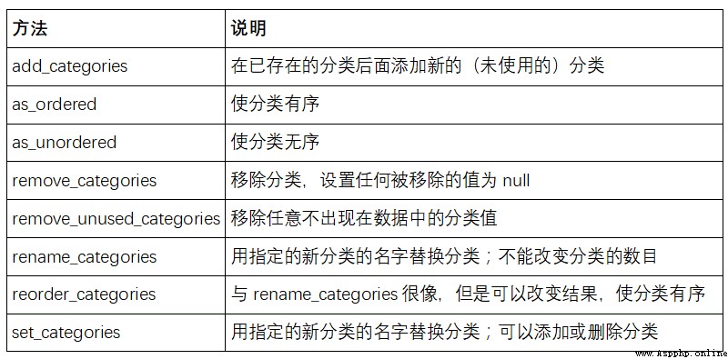
surface 12-1 Lists the available classification methods .
When you use statistics or machine learning tools , Classification data is usually converted into dummy variables , Also known as one-hot code . This includes creating a column of different categories DataFrame; These columns contain... For a given classification 1s, Others are 0.
Look at the previous example :
In [73]: cat_s = pd.Series(['a', 'b', 'c', 'd'] * 2, dtype='category')
The first one 7 Chapter mentioned ,pandas.get_dummies Function can convert the classification data to a class containing virtual variables DataFrame:
In [74]: pd.get_dummies(cat_s)
Out[74]:
a b c d
0 1 0 0 0
1 0 1 0 0
2 0 0 1 0
3 0 0 0 1
4 1 0 0 0
5 0 1 0 0
6 0 0 1 0
7 0 0 0 1
Even though we're in the third place 10 Chapter has been deeply studied Series and DataFrame Of Groupby Method , There are also some methods that are very useful .
In the 10 Chapter , We learned in grouping operation apply Method , convert . There's another one transform Method , It is associated with apply It's like , But there are certain restrictions on the functions used :
Let's take a simple example :
In [75]: df = pd.DataFrame({
'key': ['a', 'b', 'c'] * 4,
....: 'value': np.arange(12.)})
In [76]: df
Out[76]:
key value
0 a 0.0
1 b 1.0
2 c 2.0
3 a 3.0
4 b 4.0
5 c 5.0
6 a 6.0
7 b 7.0
8 c 8.0
9 a 9.0
10 b 10.0
11 c 11.0
Press the key to group :
In [77]: g = df.groupby('key').value
In [78]: g.mean()
Out[78]:
key
a 4.5
b 5.5
c 6.5
Name: value, dtype: float64
Suppose we want to generate a sum df[‘value’] Of the same shape Series, But the value is replaced by the average value of the key group . We can transfer functions lambda x: x.mean() convert :
In [79]: g.transform(lambda x: x.mean())
Out[79]:
0 4.5
1 5.5
2 6.5
3 4.5
4 5.5
5 6.5
6 4.5
7 5.5
8 6.5
9 4.5
10 5.5
11 6.5
Name: value, dtype: float64
For built-in aggregate functions , We can pass a string kana as GroupBy Of agg Method :
In [80]: g.transform('mean')
Out[80]:
0 4.5
1 5.5
2 6.5
3 4.5
4 5.5
5 6.5
6 4.5
7 5.5
8 6.5
9 4.5
10 5.5
11 6.5
Name: value, dtype: float64
And apply similar ,transform The function of will return Series, But the result must be the same size as the input . for instance , We can use lambda Function multiplies each group by 2:
In [81]: g.transform(lambda x: x * 2)
Out[81]:
0 0.0
1 2.0
2 4.0
3 6.0
4 8.0
5 10.0
6 12.0
7 14.0
8 16.0
9 18.0
10 20.0
11 22.0
Name: value, dtype: float64
Another complicated example , We can calculate the descending rank of each group :
In [82]: g.transform(lambda x: x.rank(ascending=False))
Out[82]:
0 4.0
1 4.0
2 4.0
3 3.0
4 3.0
5 3.0
6 2.0
7 2.0
8 2.0
9 1.0
10 1.0
11 1.0
Name: value, dtype: float64
Look at a grouping transformation function constructed by a simple aggregation :
def normalize(x):
return (x - x.mean()) / x.std()
We use it transform or apply Equivalent results can be obtained :
In [84]: g.transform(normalize)
Out[84]:
0 -1.161895
1 -1.161895
2 -1.161895
3 -0.387298
4 -0.387298
5 -0.387298
6 0.387298
7 0.387298
8 0.387298
9 1.161895
10 1.161895
11 1.161895
Name: value, dtype: float64
In [85]: g.apply(normalize)
Out[85]:
0 -1.161895
1 -1.161895
2 -1.161895
3 -0.387298
4 -0.387298
5 -0.387298
6 0.387298
7 0.387298
8 0.387298
9 1.161895
10 1.161895
11 1.161895
Name: value, dtype: float64
Built in aggregate functions , such as mean or sum, Often than apply Fast function , Is better than transform fast . This allows us to do a so-called unsealing (unwrapped) Grouping operation :
In [86]: g.transform('mean')
Out[86]:
0 4.5
1 5.5
2 6.5
3 4.5
4 5.5
5 6.5
6 4.5
7 5.5
8 6.5
9 4.5
10 5.5
11 6.5
Name: value, dtype: float64
In [87]: normalized = (df['value'] - g.transform('mean')) / g.transform('std')
In [88]: normalized
Out[88]:
0 -1.161895
1 -1.161895
2 -1.161895
3 -0.387298
4 -0.387298
5 -0.387298
6 0.387298
7 0.387298
8 0.387298
9 1.161895
10 1.161895
11 1.161895
Name: value, dtype: float64
Unsealing a packet operation may include multiple packet aggregations , But vectorization still brings benefits .
For time series data ,resample Method is semantically a grouping operation based on intrinsic time . Here is an example table :
In [89]: N = 15
In [90]: times = pd.date_range('2017-05-20 00:00', freq='1min', periods=N)
In [91]: df = pd.DataFrame({
'time': times,
....: 'value': np.arange(N)})
In [92]: df
Out[92]:
time value
0 2017-05-20 00:00:00 0
1 2017-05-20 00:01:00 1
2 2017-05-20 00:02:00 2
3 2017-05-20 00:03:00 3
4 2017-05-20 00:04:00 4
5 2017-05-20 00:05:00 5
6 2017-05-20 00:06:00 6
7 2017-05-20 00:07:00 7
8 2017-05-20 00:08:00 8
9 2017-05-20 00:09:00 9
10 2017-05-20 00:10:00 10
11 2017-05-20 00:11:00 11
12 2017-05-20 00:12:00 12
13 2017-05-20 00:13:00 13
14 2017-05-20 00:14:00 14
here , We can use time As index , Then resample :
In [93]: df.set_index('time').resample('5min').count()
Out[93]:
value
time
2017-05-20 00:00:00 5
2017-05-20 00:05:00 5
2017-05-20 00:10:00 5
hypothesis DataFrame Contains multiple time series , Tag with an additional column of grouping keys :
In [94]: df2 = pd.DataFrame({
'time': times.repeat(3),
....: 'key': np.tile(['a', 'b', 'c'], N),
....: 'value': np.arange(N * 3.)})
In [95]: df2[:7]
Out[95]:
key time value
0 a 2017-05-20 00:00:00 0.0
1 b 2017-05-20 00:00:00 1.0
2 c 2017-05-20 00:00:00 2.0
3 a 2017-05-20 00:01:00 3.0
4 b 2017-05-20 00:01:00 4.0
5 c 2017-05-20 00:01:00 5.0
6 a 2017-05-20 00:02:00 6.0
To each key Value for the same resample , We introduce pandas.TimeGrouper object :
In [96]: time_key = pd.TimeGrouper('5min')
We then set the time index , use key and time_key grouping , And then aggregate :
In [97]: resampled = (df2.set_index('time')
....: .groupby(['key', time_key])
....: .sum())
In [98]: resampled
Out[98]:
value
key time
a 2017-05-20 00:00:00 30.0
2017-05-20 00:05:00 105.0
2017-05-20 00:10:00 180.0
b 2017-05-20 00:00:00 35.0
2017-05-20 00:05:00 110.0
2017-05-20 00:10:00 185.0
c 2017-05-20 00:00:00 40.0
2017-05-20 00:05:00 115.0
2017-05-20 00:10:00 190.0
In [99]: resampled.reset_index()
Out[99]:
key time value
0 a 2017-05-20 00:00:00 30.0
1 a 2017-05-20 00:05:00 105.0
2 a 2017-05-20 00:10:00 180.0
3 b 2017-05-20 00:00:00 35.0
4 b 2017-05-20 00:05:00 110.0
5 b 2017-05-20 00:10:00 185.0
6 c 2017-05-20 00:00:00 40.0
7 c 2017-05-20 00:05:00 115.0
8 c 2017-05-20 00:10:00 190.0
Use TimeGrouper The limit is that the time must be Series or DataFrame The index of .
When performing a series of transformations on a dataset , You may find that the created temporary variables are not used in the analysis . See the following example :
df = load_data()
df2 = df[df['col2'] < 0]
df2['col1_demeaned'] = df2['col1'] - df2['col1'].mean()
result = df2.groupby('key').col1_demeaned.std()
Although real data is not used here , This example points out some new methods . First ,DataFrame.assign The method is a df[k] = v Form of functional column assignment method . It is not an in place modification of objects , Instead, it returns the new and modified DataFrame. therefore , The following statements are equivalent :
# Usual non-functional way
df2 = df.copy()
df2['k'] = v
# Functional assign way
df2 = df.assign(k=v)
Local distribution may be better than assign fast , however assign It is convenient to carry out chain programming :
result = (df2.assign(col1_demeaned=df2.col1 - df2.col2.mean())
.groupby('key')
.col1_demeaned.std())
I use outer parentheses , This makes it easy to add line breaks .
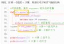
Pay attention to when using chain programming , You may need to involve temporary objects . In the previous example , We can't use load_data Result , Until it is assigned to a temporary variable df. In order to do so ,assign And many others pandas Functions can take arguments like functions , You can call the object (callable). To show callable objects , Look at a clip from the previous example :
df = load_data()
df2 = df[df['col2'] < 0]
It can be rewritten as :
df = (load_data()
[lambda x: x['col2'] < 0])
here ,load_data The result of is not assigned to a variable , So pass to [ ] The function of is bound to the object in this step .
We can write the whole process as a single chain expression :
result = (load_data()
[lambda x: x.col2 < 0]
.assign(col1_demeaned=lambda x: x.col1 - x.col1.mean())
.groupby('key')
.col1_demeaned.std())
Whether to write code in this form is just a habit , Separating it into several steps can improve readability .
You can use it. Python Built in pandas Functions and methods , Do a lot of work with chained programming with callable objects . however , Sometimes you need to use your own functions , Or third-party library functions . At this time, the pipeline method is used .
Look at the function call below :
a = f(df, arg1=v1)
b = g(a, v2, arg3=v3)
c = h(b, arg4=v4)
When using receive 、 return Series or DataFrame The functional expression of the object , You can call pipe Rewrite it :
result = (df.pipe(f, arg1=v1)
.pipe(g, v2, arg3=v3)
.pipe(h, arg4=v4))
f(df) and df.pipe(f) It is equivalent. , however pipe Make chained declarations easier .
pipe Another useful aspect of is to refine operations into reusable functions . Consider an example of subtracting a grouping method from a column :
g = df.groupby(['key1', 'key2'])
df['col1'] = df['col1'] - g.transform('mean')
Suppose you want to convert multiple columns , And modify the key of the group . in addition , You want to use chain programming to do this conversion . Here is a way :
def group_demean(df, by, cols):
result = df.copy()
g = df.groupby(by)
for c in cols:
result[c] = df[c] - g[c].transform('mean')
return result
Then it can be written as :
result = (df[df.col1 < 0]
.pipe(group_demean, ['key1', 'key2'], ['col1']))
Like many other open source projects ,pandas Still in constant change and progress . As elsewhere in this book , The focus here is on stable features that will not change in the next few years .
In order to study deeply pandas Knowledge , I suggest you study the official documents , And read the document updates released by the development team . We also invite you to join us pandas Development of : modify bug、 Create new features 、 Perfect the documentation .