Data transferred from (GitHub Address ):https://github.com/wesm/pydata-book Friends in need can go by themselves github download 
The last chapter of the book , Let's look at some real-world datasets . For each data set , We will use the method introduced before , Extract meaningful content from raw data . The method presented is applicable to other data sets , Including yours . This chapter contains a variety of case datasets , It can be used to practice .
Case datasets can be found in Github Warehouse found , See Chapter one .
#14.1 come from Bitly Of USA.gov data
2011 year ,URL Shorten service Bitly With the US government website USA.gov cooperation , Provides a copy of the generated from .gov or .mil Anonymous data collected from users with short links . stay 2011 year , In addition to real-time data , You can also download hourly snapshots in the form of text files . When writing this book (2017 year ), The service has been shut down , But we keep a copy of the data for the case of this book .
Take the hourly snapshot as an example , The format of each line in the file is JSON( namely JavaScript Object Notation, This is a common Web data format ). for example , If we only read the first line in a file , Then the result should be as follows :
In [5]: path = 'datasets/bitly_usagov/example.txt'
In [6]: open(path).readline()
Out[6]: '{
 "a": "Mozilla\\/5.0 (Windows NT 6.1; WOW64) AppleWebKit\\/535.11
(KHTML, like Gecko) Chrome\\/17.0.963.78 Safari\\/535.11", "c": "US", "nk": 1,
"tz": "America\\/New_York", "gr": "MA", "g": "A6qOVH", "h": "wfLQtf", "l":
"orofrog", "al": "en-US,en;q=0.8", "hh": "1.usa.gov", "r":
"http:\\/\\/www.facebook.com\\/l\\/7AQEFzjSi\\/1.usa.gov\\/wfLQtf", "u":
"http:\\/\\/www.ncbi.nlm.nih.gov\\/pubmed\\/22415991", "t": 1331923247, "hc":
1331822918, "cy": "Danvers", "ll": [ 42.576698, -70.954903 ] }\n'
Python There are built-in or third-party modules that can JSON The string is converted to Python A dictionary object . here , I will use json Modules and loads Function to load the downloaded data file line by line :
import json
path = 'datasets/bitly_usagov/example.txt'
records = [json.loads(line) for line in open(path)]
Now? ,records Objects become a group Python It's a dictionary :
In [18]: records[0]
Out[18]:
{
'a': 'Mozilla/5.0 (Windows NT 6.1; WOW64) AppleWebKit/535.11 (KHTML, like Gecko)
Chrome/17.0.963.78 Safari/535.11',
'al': 'en-US,en;q=0.8',
'c': 'US',
'cy': 'Danvers',
'g': 'A6qOVH',
'gr': 'MA',
'h': 'wfLQtf',
'hc': 1331822918,
'hh': '1.usa.gov',
'l': 'orofrog',
'll': [42.576698, -70.954903],
'nk': 1,
'r': 'http://www.facebook.com/l/7AQEFzjSi/1.usa.gov/wfLQtf',
't': 1331923247,
'tz': 'America/New_York',
'u': 'http://www.ncbi.nlm.nih.gov/pubmed/22415991'}
## In pure Python The code counts the time zone
Suppose we want to know which time zone appears most frequently in the dataset ( namely tz Field ), There are many ways to get the answer . First , We use list derivation to take out a set of time zones :
In [12]: time_zones = [rec['tz'] for rec in records]
---------------------------------------------------------------------------
KeyError Traceback (most recent call last)
<ipython-input-12-db4fbd348da9> in <module>()
----> 1 time_zones = [rec['tz'] for rec in records]
<ipython-input-12-db4fbd348da9> in <listcomp>(.0)
----> 1 time_zones = [rec['tz'] for rec in records]
KeyError: 'tz'
dizzy ! It turns out that not all records have time zone fields . This is easy to handle. , Just add a... To the end of the list derivation if 'tz’in rec Just judge :
In [13]: time_zones = [rec['tz'] for rec in records if 'tz' in rec]
In [14]: time_zones[:10]
Out[14]:
['America/New_York',
'America/Denver',
'America/New_York',
'America/Sao_Paulo',
'America/New_York',
'America/New_York',
'Europe/Warsaw',
'',
'',
'']
Just look at the front 10 Time zone , We find that some are unknown ( It's empty ). Although they can be filtered out , But keep it for now . Next , To count the time zone , Here are two ways : One is more difficult ( Use only standards Python library ), The other is simpler ( Use pandas). One way to count is to store the count value in a dictionary while traversing the time zone :
def get_counts(sequence):
counts = {
}
for x in sequence:
if x in counts:
counts[x] += 1
else:
counts[x] = 1
return counts
If you use Python More advanced tools for the standard library , Then you might write the code more succinctly :
from collections import defaultdict
def get_counts2(sequence):
counts = defaultdict(int) # values will initialize to 0
for x in sequence:
counts[x] += 1
return counts
I write logic into functions for greater reusability . To use it to process time zones , Just put the time_zones Just pass it in :
In [17]: counts = get_counts(time_zones)
In [18]: counts['America/New_York']
Out[18]: 1251
In [19]: len(time_zones)
Out[19]: 3440
If you want to get before 10 Bit time zone and its count value , We need to use some dictionary skills :
def top_counts(count_dict, n=10):
value_key_pairs = [(count, tz) for tz, count in count_dict.items()]
value_key_pairs.sort()
return value_key_pairs[-n:]
Then there is :
In [21]: top_counts(counts)
Out[21]:
[(33, 'America/Sao_Paulo'),
(35, 'Europe/Madrid'),
(36, 'Pacific/Honolulu'),
(37, 'Asia/Tokyo'),
(74, 'Europe/London'),
(191, 'America/Denver'),
(382, 'America/Los_Angeles'),
(400, 'America/Chicago'),
(521, ''),
(1251, 'America/New_York')]
If you search Python The standard library of , You can find collections.Counter class , It can make the job easier :
In [22]: from collections import Counter
In [23]: counts = Counter(time_zones)
In [24]: counts.most_common(10)
Out[24]:
[('America/New_York', 1251),
('', 521),
('America/Chicago', 400),
('America/Los_Angeles', 382),
('America/Denver', 191),
('Europe/London', 74),
('Asia/Tokyo', 37),
('Pacific/Honolulu', 36),
('Europe/Madrid', 35),
('America/Sao_Paulo', 33)]
Create from a collection of original records DateFrame, And pass the record list to pandas.DataFrame It's as simple as :
In [25]: import pandas as pd
In [26]: frame = pd.DataFrame(records)
In [27]: frame.info()
<class 'pandas.core.frame.DataFrame'>
RangeIndex: 3560 entries, 0 to 3559
Data columns (total 18 columns):
_heartbeat_ 120 non-null float64
a 3440 non-null object
al 3094 non-null object
c 2919 non-null object
cy 2919 non-null object
g 3440 non-null object
gr 2919 non-null object
h 3440 non-null object
hc 3440 non-null float64
hh 3440 non-null object
kw 93 non-null object
l 3440 non-null object
ll 2919 non-null object
nk 3440 non-null float64
r 3440 non-null object
t 3440 non-null float64
tz 3440 non-null object
u 3440 non-null object
dtypes: float64(4), object(14)
memory usage: 500.7+ KB
In [28]: frame['tz'][:10]
Out[28]:
0 America/New_York
1 America/Denver
2 America/New_York
3 America/Sao_Paulo
4 America/New_York
5 America/New_York
6 Europe/Warsaw
7
8
9
Name: tz, dtype: object
here frame The output form of is the summary view (summary view), Mainly used for larger DataFrame object . We can then talk about Series Use value_counts Method :
In [29]: tz_counts = frame['tz'].value_counts()
In [30]: tz_counts[:10]
Out[30]:
America/New_York 1251
521
America/Chicago 400
America/Los_Angeles 382
America/Denver 191
Europe/London 74
Asia/Tokyo 37
Pacific/Honolulu 36
Europe/Madrid 35
America/Sao_Paulo 33
Name: tz, dtype: int64
We can use matplotlib Visualize this data . So , Let's first fill in an alternative value for the unknown or missing time zone in the record .fillna Function can replace missing values (NA), And unknown value ( An empty string ) Can be replaced by a Boolean array index :
In [31]: clean_tz = frame['tz'].fillna('Missing')
In [32]: clean_tz[clean_tz == ''] = 'Unknown'
In [33]: tz_counts = clean_tz.value_counts()
In [34]: tz_counts[:10]
Out[34]:
America/New_York 1251
Unknown 521
America/Chicago 400
America/Los_Angeles 382
America/Denver 191
Missing 120
Europe/London 74
Asia/Tokyo 37
Pacific/Honolulu 36
Europe/Madrid 35
Name: tz, dtype: int64
here , We can use seaborn Package create horizontal histogram ( The results are shown in the figure 14-1):
In [36]: import seaborn as sns
In [37]: subset = tz_counts[:10]
In [38]: sns.barplot(y=subset.index, x=subset.values)
a The field contains execution URL Browser for shortening operation 、 equipment 、 Information about the application :
In [39]: frame['a'][1]
Out[39]: 'GoogleMaps/RochesterNY'
In [40]: frame['a'][50]
Out[40]: 'Mozilla/5.0 (Windows NT 5.1; rv:10.0.2)
Gecko/20100101 Firefox/10.0.2'
In [41]: frame['a'][51][:50] # long line
Out[41]: 'Mozilla/5.0 (Linux; U; Android 2.2.2; en-us; LG-P9'
Will these "agent" Parsing all the information in a string is a frustrating job . One strategy is to put the first section of this string ( Roughly corresponding to the browser ) Isolate and get another summary of user behavior :
In [42]: results = pd.Series([x.split()[0] for x in frame.a.dropna()])
In [43]: results[:5]
Out[43]:
0 Mozilla/5.0
1 GoogleMaps/RochesterNY
2 Mozilla/4.0
3 Mozilla/5.0
4 Mozilla/5.0
dtype: object
In [44]: results.value_counts()[:8]
Out[44]:
Mozilla/5.0 2594
Mozilla/4.0 601
GoogleMaps/RochesterNY 121
Opera/9.80 34
TEST_INTERNET_AGENT 24
GoogleProducer 21
Mozilla/6.0 5
BlackBerry8520/5.0.0.681 4
dtype: int64
Now? , Suppose you want to press Windows He Fei Windows The user decomposes the time zone statistics . For the sake of simplicity , We assume that as long as agent The string contains "Windows" It is considered that the user is Windows user . Because there are agent defect , So first remove them from the data :
In [45]: cframe = frame[frame.a.notnull()]
Then calculate whether each row contains Windows Value :
In [47]: cframe['os'] = np.where(cframe['a'].str.contains('Windows'),
....: 'Windows', 'Not Windows')
In [48]: cframe['os'][:5]
Out[48]:
0 Windows
1 Not Windows
2 Windows
3 Not Windows
4 Windows
Name: os, dtype: object
Next, you can group the data according to the time zone and the newly obtained operating system list :
In [49]: by_tz_os = cframe.groupby(['tz', 'os'])
Group count , Be similar to value_counts function , It can be used size To calculate . And make use of unstack Reshape the counting results :
In [50]: agg_counts = by_tz_os.size().unstack().fillna(0)
In [51]: agg_counts[:10]
Out[51]:
os Not Windows Windows
tz
245.0 276.0
Africa/Cairo 0.0 3.0
Africa/Casablanca 0.0 1.0
Africa/Ceuta 0.0 2.0
Africa/Johannesburg 0.0 1.0
Africa/Lusaka 0.0 1.0
America/Anchorage 4.0 1.0
America/Argentina/Buenos_Aires 1.0 0.0
America/Argentina/Cordoba 0.0 1.0
America/Argentina/Mendoza 0.0 1.0
Last , Let's choose the most common time zone . In order to achieve this goal , I base agg_counts The number of rows in constructs an indirect index array :
# Use to sort in ascending order
In [52]: indexer = agg_counts.sum(1).argsort()
In [53]: indexer[:10]
Out[53]:
tz
24
Africa/Cairo 20
Africa/Casablanca 21
Africa/Ceuta 92
Africa/Johannesburg 87
Africa/Lusaka 53
America/Anchorage 54
America/Argentina/Buenos_Aires 57
America/Argentina/Cordoba 26
America/Argentina/Mendoza 55
dtype: int64
Then I go through take In this order, the last 10 Line maximum :
In [54]: count_subset = agg_counts.take(indexer[-10:])
In [55]: count_subset
Out[55]:
os Not Windows Windows
tz
America/Sao_Paulo 13.0 20.0
Europe/Madrid 16.0 19.0
Pacific/Honolulu 0.0 36.0
Asia/Tokyo 2.0 35.0
Europe/London 43.0 31.0
America/Denver 132.0 59.0
America/Los_Angeles 130.0 252.0
America/Chicago 115.0 285.0
245.0 276.0
America/New_York 339.0 912.0
pandas There's a simple way nlargest, Can do the same job :
In [56]: agg_counts.sum(1).nlargest(10)
Out[56]:
tz
America/New_York 1251.0
521.0
America/Chicago 400.0
America/Los_Angeles 382.0
America/Denver 191.0
Europe/London 74.0
Asia/Tokyo 37.0
Pacific/Honolulu 36.0
Europe/Madrid 35.0
America/Sao_Paulo 33.0
dtype: float64
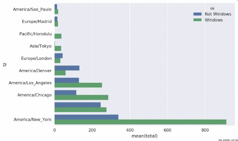
then , As this code shows , Can be represented by histogram . I pass an extra parameter to seaborn Of barpolt function , To draw a stacked bar chart ( See the picture 14-2):
# Rearrange the data for plotting
In [58]: count_subset = count_subset.stack()
In [59]: count_subset.name = 'total'
In [60]: count_subset = count_subset.reset_index()
In [61]: count_subset[:10]
Out[61]:
tz os total
0 America/Sao_Paulo Not Windows 13.0
1 America/Sao_Paulo Windows 20.0
2 Europe/Madrid Not Windows 16.0
3 Europe/Madrid Windows 19.0
4 Pacific/Honolulu Not Windows 0.0
5 Pacific/Honolulu Windows 36.0
6 Asia/Tokyo Not Windows 2.0
7 Asia/Tokyo Windows 35.0
8 Europe/London Not Windows 43.0
9 Europe/London Windows 31.0
In [62]: sns.barplot(x='total', y='tz', hue='os', data=count_subset)
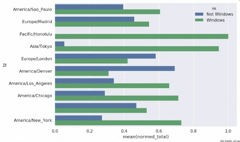
This picture is not easy to see Windows The relative proportion of users in small groups , Therefore, the sum of the percentage of standardized groups is 1:
def norm_total(group):
group['normed_total'] = group.total / group.total.sum()
return group
results = count_subset.groupby('tz').apply(norm_total)
Draw again , See the picture 14-3:
In [65]: sns.barplot(x='normed_total', y='tz', hue='os', data=results)
We can still use it groupby Of transform Method , More efficient computation of standardized and :
In [66]: g = count_subset.groupby('tz')
In [67]: results2 = count_subset.total / g.total.transform('sum')
GroupLens Research(http://www.grouplens.org/node/73) Collected a group from 20 century 90 By the end of the year 21 At the beginning of the century MovieLens Movie rating data provided by users . These figures include movie ratings 、 Movie metadata ( Style type and age ) And demographic data about users ( Age 、 Zip code 、 Gender and occupation, etc ). Recommendation systems based on machine learning algorithms are generally interested in such data . Although I will not introduce machine learning technology in detail in this book , But I will show you how to slice and dice this data to meet the actual needs .
MovieLens 1M The dataset contains data from 6000 User pair 4000 Of a movie 100 10000 scoring data . It is divided into three tables : score 、 User information and movie information . Take the data from zip After extracting the file , Can pass pandas.read_table Read each table to a pandas DataFrame In the object :
import pandas as pd
# Make display smaller
pd.options.display.max_rows = 10
unames = ['user_id', 'gender', 'age', 'occupation', 'zip']
users = pd.read_table('datasets/movielens/users.dat', sep='::',
header=None, names=unames)
rnames = ['user_id', 'movie_id', 'rating', 'timestamp']
ratings = pd.read_table('datasets/movielens/ratings.dat', sep='::',
header=None, names=rnames)
mnames = ['movie_id', 'title', 'genres']
movies = pd.read_table('datasets/movielens/movies.dat', sep='::',
header=None, names=mnames)
utilize Python Slicing syntax for , By viewing each DataFrame The first few lines of can be used to verify whether the data loading is going well :
In [69]: users[:5]
Out[69]:
user_id gender age occupation zip
0 1 F 1 10 48067
1 2 M 56 16 70072
2 3 M 25 15 55117
3 4 M 45 7 02460
4 5 M 25 20 55455
In [70]: ratings[:5]
Out[70]:
user_id movie_id rating timestamp
0 1 1193 5 978300760
1 1 661 3 978302109
2 1 914 3 978301968
3 1 3408 4 978300275
4 1 2355 5 978824291
In [71]: movies[:5]
Out[71]:
movie_id title genres
0 1 Toy Story (1995) Animation|Children's|Comedy
1 2 Jumanji (1995) Adventure|Children's|Fantasy
2 3 Grumpier Old Men (1995) Comedy|Romance
3 4 Waiting to Exhale (1995) Comedy|Drama
4 5 Father of the Bride Part II (1995) Comedy
In [72]: ratings
Out[72]:
user_id movie_id rating timestamp
0 1 1193 5 978300760
1 1 661 3 978302109
2 1 914 3 978301968
3 1 3408 4 978300275
4 1 2355 5 978824291
... ... ... ... ...
1000204 6040 1091 1 956716541
1000205 6040 1094 5 956704887
1000206 6040 562 5 956704746
1000207 6040 1096 4 956715648
1000208 6040 1097 4 956715569
[1000209 rows x 4 columns]
Be careful , The age and occupation are given in coded form , For their specific meanings, please refer to the README file . It is not easy to analyze the data scattered in three tables . Suppose we want to calculate the average score of a movie based on sex and age , It would be much easier to merge all the data into one table . We use first pandas Of merge Function will ratings Follow users Merge together , And then movies Also incorporated .pandas It will infer which columns are merged according to the overlap of column names ( Or connection ) key :
In [73]: data = pd.merge(pd.merge(ratings, users), movies)
In [74]: data
Out[74]:
user_id movie_id rating timestamp gender age occupation zip \
0 1 1193 5 978300760 F 1 10 48067
1 2 1193 5 978298413 M 56 16 70072
2 12 1193 4 978220179 M 25 12 32793
3 15 1193 4 978199279 M 25 7 22903
4 17 1193 5 978158471 M 50 1 95350
... ... ... ... ... ... ... ... ...
1000204 5949 2198 5 958846401 M 18 17 47901
1000205 5675 2703 3 976029116 M 35 14 30030
1000206 5780 2845 1 958153068 M 18 17 92886
1000207 5851 3607 5 957756608 F 18 20 55410
1000208 5938 2909 4 957273353 M 25 1 35401
title genres
0 One Flew Over the Cuckoo's Nest (1975) Drama
1 One Flew Over the Cuckoo's Nest (1975) Drama
2 One Flew Over the Cuckoo's Nest (1975) Drama
3 One Flew Over the Cuckoo's Nest (1975) Drama
4 One Flew Over the Cuckoo's Nest (1975) Drama
... ... ...
1000204 Modulations (1998) Documentary
1000205 Broken Vessels (1998) Drama
1000206 White Boys (1999) Drama
1000207 One Little Indian (1973) Comedy|Drama|Western
1000208 Five Wives, Three Secretaries and Me (1998) Documentary
[1000209 rows x 10 columns]
In [75]: data.iloc[0]
Out[75]:
user_id 1
movie_id 1193
rating 5
timestamp 978300760
gender F
age 1
occupation 10
zip 48067
title One Flew Over the Cuckoo's Nest (1975)
genres Drama
Name: 0, dtype: object
To calculate the average score of each film by sex , We can use pivot_table Method :
In [76]: mean_ratings = data.pivot_table('rating', index='title',
....: columns='gender', aggfunc='mean')
In [77]: mean_ratings[:5]
Out[77]:
gender F M
title
$1,000,000 Duck (1971) 3.375000 2.761905
'Night Mother (1986) 3.388889 3.352941
'Til There Was You (1997) 2.675676 2.733333
'burbs, The (1989) 2.793478 2.962085
...And Justice for All (1979) 3.828571 3.689024
This operation produces another DataFrame, The content is the average score of the film , The line is marked with the movie name ( Indexes ), The column is marked with gender . Now? , I'm going to filter out the scoring data 250 The movie of the bar ( A random number ). In order to achieve this goal , I'll be right first title Grouping , And then use it size() Get a Series object :
In [78]: ratings_by_title = data.groupby('title').size()
In [79]: ratings_by_title[:10]
Out[79]:
title
$1,000,000 Duck (1971) 37
'Night Mother (1986) 70
'Til There Was You (1997) 52
'burbs, The (1989) 303
...And Justice for All (1979) 199
1-900 (1994) 2
10 Things I Hate About You (1999) 700
101 Dalmatians (1961) 565
101 Dalmatians (1996) 364
12 Angry Men (1957) 616
dtype: int64
In [80]: active_titles = ratings_by_title.index[ratings_by_title >= 250]
In [81]: active_titles
Out[81]:
Index([''burbs, The (1989)', '10 Things I Hate About You (1999)',
'101 Dalmatians (1961)', '101 Dalmatians (1996)', '12 Angry Men (1957)',
'13th Warrior, The (1999)', '2 Days in the Valley (1996)',
'20,000 Leagues Under the Sea (1954)', '2001: A Space Odyssey (1968)',
'2010 (1984)',
...
'X-Men (2000)', 'Year of Living Dangerously (1982)',
'Yellow Submarine (1968)', 'You've Got Mail (1998)',
'Young Frankenstein (1974)', 'Young Guns (1988)',
'Young Guns II (1990)', 'Young Sherlock Holmes (1985)',
'Zero Effect (1998)', 'eXistenZ (1999)'],
dtype='object', name='title', length=1216)
The score data in the title index is greater than 250 The title of the movie , Then we can start from the previous mean_ratings Select the desired row in the :
# Select rows on the index
In [82]: mean_ratings = mean_ratings.loc[active_titles]
In [83]: mean_ratings
Out[83]:
gender F M
title
'burbs, The (1989) 2.793478 2.962085
10 Things I Hate About You (1999) 3.646552 3.311966
101 Dalmatians (1961) 3.791444 3.500000
101 Dalmatians (1996) 3.240000 2.911215
12 Angry Men (1957) 4.184397 4.328421
... ... ...
Young Guns (1988) 3.371795 3.425620
Young Guns II (1990) 2.934783 2.904025
Young Sherlock Holmes (1985) 3.514706 3.363344
Zero Effect (1998) 3.864407 3.723140
eXistenZ (1999) 3.098592 3.289086
[1216 rows x 2 columns]
To learn about the favorite movies of female audiences , We can F The columns are arranged in descending order :
In [85]: top_female_ratings = mean_ratings.sort_values(by='F', ascending=False)
In [86]: top_female_ratings[:10]
Out[86]:
gender F M
title
Close Shave, A (1995) 4.644444 4.473795
Wrong Trousers, The (1993) 4.588235 4.478261
Sunset Blvd. (a.k.a. Sunset Boulevard) (1950) 4.572650 4.464589
Wallace & Gromit: The Best of Aardman Animation... 4.563107 4.385075
Schindler's List (1993) 4.562602 4.491415
Shawshank Redemption, The (1994) 4.539075 4.560625
Grand Day Out, A (1992) 4.537879 4.293255
To Kill a Mockingbird (1962) 4.536667 4.372611
Creature Comforts (1990) 4.513889 4.272277
Usual Suspects, The (1995) 4.513317 4.518248
Suppose we want to find out which movies have the most divergent male and female audiences . One way is to give mean_ratings Add a column for storing the difference between the average scores , And sort it :
In [87]: mean_ratings['diff'] = mean_ratings['M'] - mean_ratings['F']
Press "diff" Then you can get the most divergent movies that female audiences prefer :
In [88]: sorted_by_diff = mean_ratings.sort_values(by='diff')
In [89]: sorted_by_diff[:10]
Out[89]:
gender F M diff
title
Dirty Dancing (1987) 3.790378 2.959596 -0.830782
Jumpin' Jack Flash (1986) 3.254717 2.578358 -0.676359
Grease (1978) 3.975265 3.367041 -0.608224
Little Women (1994) 3.870588 3.321739 -0.548849
Steel Magnolias (1989) 3.901734 3.365957 -0.535777
Anastasia (1997) 3.800000 3.281609 -0.518391
Rocky Horror Picture Show, The (1975) 3.673016 3.160131 -0.512885
Color Purple, The (1985) 4.158192 3.659341 -0.498851
Age of Innocence, The (1993) 3.827068 3.339506 -0.487561
Free Willy (1993) 2.921348 2.438776 -0.482573
Reverse the order of the sorting results and take out the previous 10 That's ok , What you get is a movie that male audiences prefer :
# Reverse order of rows, take first 10 rows
In [90]: sorted_by_diff[::-1][:10]
Out[90]:
gender F M diff
title
Good, The Bad and The Ugly, The (1966) 3.494949 4.221300 0.726351
Kentucky Fried Movie, The (1977) 2.878788 3.555147 0.676359
Dumb & Dumber (1994) 2.697987 3.336595 0.638608
Longest Day, The (1962) 3.411765 4.031447 0.619682
Cable Guy, The (1996) 2.250000 2.863787 0.613787
Evil Dead II (Dead By Dawn) (1987) 3.297297 3.909283 0.611985
Hidden, The (1987) 3.137931 3.745098 0.607167
Rocky III (1982) 2.361702 2.943503 0.581801
Caddyshack (1980) 3.396135 3.969737 0.573602
For a Few Dollars More (1965) 3.409091 3.953795 0.544704
If you just want to find the most divergent movies ( Regardless of gender ), The variance or standard deviation of the score data can be calculated :
# Standard deviation of rating grouped by title
In [91]: rating_std_by_title = data.groupby('title')['rating'].std()
# Filter down to active_titles
In [92]: rating_std_by_title = rating_std_by_title.loc[active_titles]
# Order Series by value in descending order
In [93]: rating_std_by_title.sort_values(ascending=False)[:10]
Out[93]:
title
Dumb & Dumber (1994) 1.321333
Blair Witch Project, The (1999) 1.316368
Natural Born Killers (1994) 1.307198
Tank Girl (1995) 1.277695
Rocky Horror Picture Show, The (1975) 1.260177
Eyes Wide Shut (1999) 1.259624
Evita (1996) 1.253631
Billy Madison (1995) 1.249970
Fear and Loathing in Las Vegas (1998) 1.246408
Bicentennial Man (1999) 1.245533
Name: rating, dtype: float64
Maybe you've noticed , Film classification is based on vertical lines (|) Given as a delimited string . If you want to analyze the film classification , You need to convert it into a more useful form first .
United States social security administration (SSA) Provided a copy from 1880 Baby name frequency data from to now .Hadley Wickham( A lot of fashion R The author of the package ) This data is often used to demonstrate R Data processing function .
We need to do some data warping to load this dataset , Doing so will result in the following DataFrame:
In [4]: names.head(10)
Out[4]:
name sex births year
0 Mary F 7065 1880
1 Anna F 2604 1880
2 Emma F 2003 1880
3 Elizabeth F 1939 1880
4 Minnie F 1746 1880
5 Margaret F 1578 1880
6 Ida F 1472 1880
7 Alice F 1414 1880
8 Bertha F 1320 1880
9 Sarah F 1288 1880
You can do many things with this data set , for example :
Use the tools described above , These analyses can be done easily , I will explain some of them .
At the time of writing this book , The United States social security administration has made the database into several data files on an annual basis , Each gender is given / The total number of births in the name group . The original files of these documents can be obtained here :http://www.ssa.gov/oact/babynames/limits.html.
If this page is missing when you read this book , You can also use the search engine to find .
download "National data" file names.zip, The extracted directory contains a set of files ( Such as yob1880.txt). I use UNIX Of head The command looks at the top of one of the files 10 That's ok ( stay Windows On , You can use it. more command , Or open it directly in a text editor ):
In [94]: !head -n 10 datasets/babynames/yob1880.txt
Mary,F,7065
Anna,F,2604
Emma,F,2003
Elizabeth,F,1939
Minnie,F,1746
Margaret,F,1578
Ida,F,1472
Alice,F,1414
Bertha,F,1320
Sarah,F,1288
Because this is a very standard comma separated format , So it can be used pandas.read_csv Load it into DataFrame in :
In [95]: import pandas as pd
In [96]: names1880 =
pd.read_csv('datasets/babynames/yob1880.txt',
....: names=['name', 'sex', 'births'])
In [97]: names1880
Out[97]:
name sex births
0 Mary F 7065
1 Anna F 2604
2 Emma F 2003
3 Elizabeth F 1939
4 Minnie F 1746
... ... .. ...
1995 Woodie M 5
1996 Worthy M 5
1997 Wright M 5
1998 York M 5
1999 Zachariah M 5
[2000 rows x 3 columns]
These documents contain only those that appear in the current year in excess of 5 My name . For the sake of simplicity , We can use births Column sex The sub total of the group represents the births A total of :
In [98]: names1880.groupby('sex').births.sum()
Out[98]:
sex
F 90993
M 110493
Name: births, dtype: int64
Because the dataset is divided into multiple files by year , So the first thing is to assemble all the data into one DataFrame Inside , And add a year Field . Use pandas.concat That's how it works :
years = range(1880, 2011)
pieces = []
columns = ['name', 'sex', 'births']
for year in years:
path = 'datasets/babynames/yob%d.txt' % year
frame = pd.read_csv(path, names=columns)
frame['year'] = year
pieces.append(frame)
# Concatenate everything into a single DataFrame
names = pd.concat(pieces, ignore_index=True)
Here are a few things to note . First of all ,concat The default is multiple by line DataFrame Put together ; second , Must specify ignore_index=True, Because we don't want to keep read_csv The original line number returned . Now we have a very big DataFrame, It contains all the name data :
In [100]: names
Out[100]:
name sex births year
0 Mary F 7065 1880
1 Anna F 2604 1880
2 Emma F 2003 1880
3 Elizabeth F 1939 1880
4 Minnie F 1746 1880
... ... .. ... ...
1690779 Zymaire M 5 2010
1690780 Zyonne M 5 2010
1690781 Zyquarius M 5 2010
1690782 Zyran M 5 2010
1690783 Zzyzx M 5 2010
[1690784 rows x 4 columns]
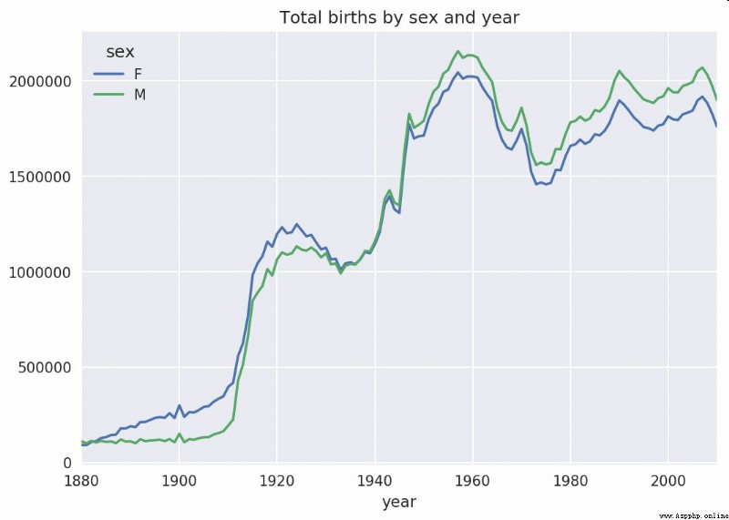
So with that data , We can use it groupby or pivot_table stay year and sex It is aggregated on the level , Pictured 14-4 Shown :
In [101]: total_births = names.pivot_table('births', index='year',
.....: columns='sex', aggfunc=sum)
In [102]: total_births.tail()
Out[102]:
sex F M
year
2006 1896468 2050234
2007 1916888 2069242
2008 1883645 2032310
2009 1827643 1973359
2010 1759010 1898382
In [103]: total_births.plot(title='Total births by sex and year')
Let's insert a prop Column , The ratio of the number of babies with a given name to the total number of births .prop The value is 0.02 each 100 Of the babies 2 Name takes the current name . therefore , Let's press first year and sex grouping , Then add the new column to each group :
def add_prop(group):
group['prop'] = group.births / group.births.sum()
return group
names = names.groupby(['year', 'sex']).apply(add_prop)
Now? , The complete dataset has the following columns :
In [105]: names
Out[105]:
name sex births year prop
0 Mary F 7065 1880 0.077643
1 Anna F 2604 1880 0.028618
2 Emma F 2003 1880 0.022013
3 Elizabeth F 1939 1880 0.021309
4 Minnie F 1746 1880 0.019188
... ... .. ... ... ...
1690779 Zymaire M 5 2010 0.000003
1690780 Zyonne M 5 2010 0.000003
1690781 Zyquarius M 5 2010 0.000003
1690782 Zyran M 5 2010 0.000003
1690783 Zzyzx M 5 2010 0.000003
[1690784 rows x 5 columns]
When such grouping processing is performed , Generally, some effectiveness checks should be done , For example, verify that all groups have prop Whether the sum of is 1:
In [106]: names.groupby(['year', 'sex']).prop.sum()
Out[106]:
year sex
1880 F 1.0
M 1.0
1881 F 1.0
M 1.0
1882 F 1.0
...
2008 M 1.0
2009 F 1.0
M 1.0
2010 F 1.0
M 1.0
Name: prop, Length: 262, dtype: float64
completion of jobs . To facilitate further analysis , I need to extract a subset of this data : Each pair sex/year Before the combination 1000 A name . This is another grouping operation :
def get_top1000(group):
return group.sort_values(by='births', ascending=False)[:1000]
grouped = names.groupby(['year', 'sex'])
top1000 = grouped.apply(get_top1000)
# Drop the group index, not needed
top1000.reset_index(inplace=True, drop=True)
If you like DIY Words , You can do that :
pieces = []
for year, group in names.groupby(['year', 'sex']):
pieces.append(group.sort_values(by='births', ascending=False)[:1000])
top1000 = pd.concat(pieces, ignore_index=True)
Now the result data set is much smaller :
In [108]: top1000
Out[108]:
name sex births year prop
0 Mary F 7065 1880 0.077643
1 Anna F 2604 1880 0.028618
2 Emma F 2003 1880 0.022013
3 Elizabeth F 1939 1880 0.021309
4 Minnie F 1746 1880 0.019188
... ... .. ... ... ...
261872 Camilo M 194 2010 0.000102
261873 Destin M 194 2010 0.000102
261874 Jaquan M 194 2010 0.000102
261875 Jaydan M 194 2010 0.000102
261876 Maxton M 193 2010 0.000102
[261877 rows x 5 columns]
The next data analysis work is aimed at this top1000 The data set .
With the complete data set and just generated top1000 Data sets , We can start analyzing various naming trends . First of all, put the front 1000 The names are divided into male and female parts :
In [109]: boys = top1000[top1000.sex == 'M']
In [110]: girls = top1000[top1000.sex == 'F']
These are two simple time series , The corresponding chart can be drawn with a little sorting ( For example, every year is called John and Mary Number of babies ). Our husband formed a press year and name A pivot table of the total number of births :
In [111]: total_births = top1000.pivot_table('births', index='year',
.....: columns='name',
.....: aggfunc=sum)
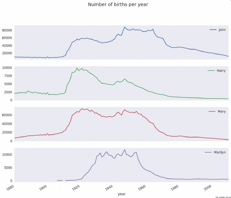
Now? , We use it DataFrame Of plot Method to draw a graph of several names ( See the picture 14-5):
In [112]: total_births.info()
<class 'pandas.core.frame.DataFrame'>
Int64Index: 131 entries, 1880 to 2010
Columns: 6868 entries, Aaden to Zuri
dtypes: float64(6868)
memory usage: 6.9 MB
In [113]: subset = total_births[['John', 'Harry', 'Mary', 'Marilyn']]
In [114]: subset.plot(subplots=True, figsize=(12, 10), grid=False,
.....: title="Number of births per year")
As you can see from the diagram , These names are no longer popular in the minds of the American people . But it's not that simple , We'll see what happened in the next section .
One explanation is that parents are willing to give their children fewer and fewer common names . This assumption can be verified from the data . One way is to calculate the most popular 1000 The proportion of names , I press year and sex Aggregate and plot ( See the picture 14-6):
In [116]: table = top1000.pivot_table('prop', index='year',
.....: columns='sex', aggfunc=sum)
In [117]: table.plot(title='Sum of table1000.prop by year and sex',
.....: yticks=np.linspace(0, 1.2, 13), xticks=range(1880, 2020, 10)
)
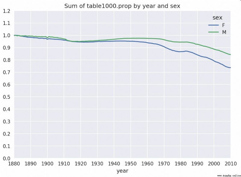
As you can see from the diagram , The diversity of names has indeed increased ( front 1000 The proportion of items decreased ). Another method is to calculate the proportion of the total number of births 50% The number of different names , This figure is not easy to calculate . Let's just think about 2010 The name of the young boy :
In [118]: df = boys[boys.year == 2010]
In [119]: df
Out[119]:
name sex births year prop
260877 Jacob M 21875 2010 0.011523
260878 Ethan M 17866 2010 0.009411
260879 Michael M 17133 2010 0.009025
260880 Jayden M 17030 2010 0.008971
260881 William M 16870 2010 0.008887
... ... .. ... ... ...
261872 Camilo M 194 2010 0.000102
261873 Destin M 194 2010 0.000102
261874 Jaquan M 194 2010 0.000102
261875 Jaydan M 194 2010 0.000102
261876 Maxton M 193 2010 0.000102
[1000 rows x 5 columns]
In the face of prop After descending , We want to know how many names in front of us add up to enough people 50%. Although write a for Circulation can indeed achieve its goal , but NumPy There's a smarter vector approach . To calculate prop The cumulative sum of cumsum, And then through searchsorted Find out 0.5 Where should it be inserted to ensure that the sequence is not broken :
In [120]: prop_cumsum = df.sort_values(by='prop', ascending=False).prop.cumsum()
In [121]: prop_cumsum[:10]
Out[121]:
260877 0.011523
260878 0.020934
260879 0.029959
260880 0.038930
260881 0.047817
260882 0.056579
260883 0.065155
260884 0.073414
260885 0.081528
260886 0.089621
Name: prop, dtype: float64
In [122]: prop_cumsum.values.searchsorted(0.5)
Out[122]: 116
Because the array index is from 0 At the beginning , So we're going to add... To this result 1, That is, the final result is 117. take 1900 To make a comparison with the data of , This number is much smaller :
In [123]: df = boys[boys.year == 1900]
In [124]: in1900 = df.sort_values(by='prop', ascending=False).prop.cumsum()
In [125]: in1900.values.searchsorted(0.5) + 1
Out[125]: 25
You can do it now for all year/sex The combination performs this calculation . Press these two fields groupby Handle , Then a function is used to calculate the value of each group :
def get_quantile_count(group, q=0.5):
group = group.sort_values(by='prop', ascending=False)
return group.prop.cumsum().values.searchsorted(q) + 1
diversity = top1000.groupby(['year', 'sex']).apply(get_quantile_count)
diversity = diversity.unstack('sex')
Now? ,diversity This DataFrame Have two time series ( One for each sex , Index by year ). adopt IPython, You can view its contents , You can also draw charts as before ( Pictured 14-7 Shown ):
In [128]: diversity.head()
Out[128]:
sex F M
year
1880 38 14
1881 38 14
1882 38 15
1883 39 15
1884 39 16
In [129]: diversity.plot(title="Number of popular names in top 50%")
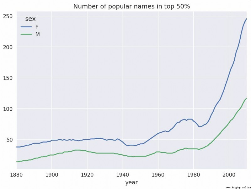
As you can see from the diagram , The diversity of girls' names is always higher than that of boys , And it's getting higher and higher . Readers can analyze for themselves what is driving this diversity ( Such as the change of spelling form ).
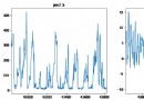
2007 year , A baby name researcher Laura Wattenberg Point out on her own website (http://www.babynamewizard.com): In the past hundred years , The distribution of boys' names on the last letter has changed significantly . In order to understand the specific situation , I first put all the birth data in the annual 、 The gender and the final letter are aggregated :
# extract last letter from name column
get_last_letter = lambda x: x[-1]
last_letters = names.name.map(get_last_letter)
last_letters.name = 'last_letter'
table = names.pivot_table('births', index=last_letters,
columns=['sex', 'year'], aggfunc=sum)
then , I have chosen a representative three years , And output the first few lines :
In [131]: subtable = table.reindex(columns=[1910, 1960, 2010], level='year')
In [132]: subtable.head()
Out[132]:
sex F M
year 1910 1960 2010 1910 1960 2010
last_letter
a 108376.0 691247.0 670605.0 977.0 5204.0 28438.0
b NaN 694.0 450.0 411.0 3912.0 38859.0
c 5.0 49.0 946.0 482.0 15476.0 23125.0
d 6750.0 3729.0 2607.0 22111.0 262112.0 44398.0
e 133569.0 435013.0 313833.0 28655.0 178823.0 129012.0
Next, we need to normalize the table according to the total number of births , So as to calculate the proportion of each gender and each last letter in the total number of births :
In [133]: subtable.sum()
Out[133]:
sex year
F 1910 396416.0
1960 2022062.0
2010 1759010.0
M 1910 194198.0
1960 2132588.0
2010 1898382.0
dtype: float64
In [134]: letter_prop = subtable / subtable.sum()
In [135]: letter_prop
Out[135]:
sex F M
year 1910 1960 2010 1910 1960 2010
last_letter
a 0.273390 0.341853 0.381240 0.005031 0.002440 0.014980
b NaN 0.000343 0.000256 0.002116 0.001834 0.020470
c 0.000013 0.000024 0.000538 0.002482 0.007257 0.012181
d 0.017028 0.001844 0.001482 0.113858 0.122908 0.023387
e 0.336941 0.215133 0.178415 0.147556 0.083853 0.067959
... ... ... ... ... ... ...
v NaN 0.000060 0.000117 0.000113
0.000037 0.001434
w 0.000020 0.000031 0.001182 0.006329 0.007711 0.016148
x 0.000015 0.000037 0.000727 0.003965 0.001851 0.008614
y 0.110972 0.152569 0.116828 0.077349 0.160987 0.058168
z 0.002439 0.000659 0.000704 0.000170 0.000184 0.001831
[26 rows x 6 columns]
With this alphanumeric data , You can generate a bar chart for each year and gender , Pictured 14-8 Shown :
import matplotlib.pyplot as plt
fig, axes = plt.subplots(2, 1, figsize=(10, 8))
letter_prop['M'].plot(kind='bar', rot=0, ax=axes[0], title='Male')
letter_prop['F'].plot(kind='bar', rot=0, ax=axes[1], title='Female',
legend=False)
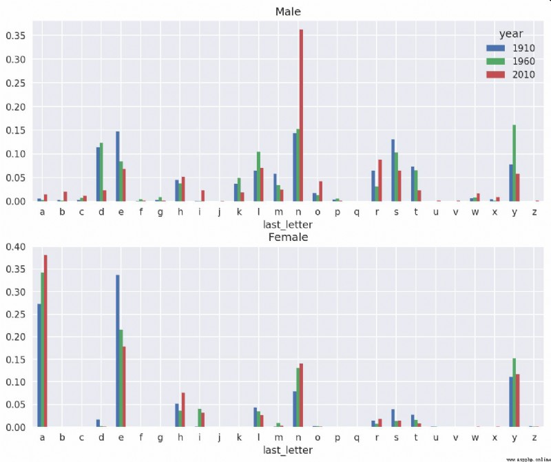
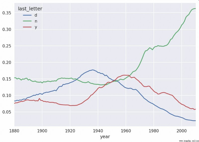
It can be seen that , from 20 century 60 s , In letters "n" There is a significant increase in the boy's name at the end . Go back to the complete table created before , It is standardized by year and gender , And choose a few letters in the boy's name , Finally, transpose to make each column into a time series :
In [138]: letter_prop = table / table.sum()
In [139]: dny_ts = letter_prop.loc[['d', 'n', 'y'], 'M'].T
In [140]: dny_ts.head()
Out[140]:
last_letter d n y
year
1880 0.083055 0.153213 0.075760
1881 0.083247 0.153214 0.077451
1882 0.085340 0.149560 0.077537
1883 0.084066 0.151646 0.079144
1884 0.086120 0.149915 0.080405
With this time series DataFrame after , Through its plot Method to draw a trend chart ( Pictured 14-9 Shown ):
In [143]: dny_ts.plot()
Another interesting trend is , The names that were popular among boys in early years have been popular in recent years “ Transsexual ”, for example Lesley or Leslie. go back to top1000 Data sets , Find out which of them is "lesl" The first group of names :
In [144]: all_names = pd.Series(top1000.name.unique())
In [145]: lesley_like = all_names[all_names.str.lower().str.contains('lesl')]
In [146]: lesley_like
Out[146]:
632 Leslie
2294 Lesley
4262 Leslee
4728 Lesli
6103 Lesly
dtype: object
Then use this result to filter other names , Count the number of births by name and check the relative frequency :
In [147]: filtered = top1000[top1000.name.isin(lesley_like)]
In [148]: filtered.groupby('name').births.sum()
Out[148]:
name
Leslee 1082
Lesley 35022
Lesli 929
Leslie 370429
Lesly 10067
Name: births, dtype: int64
Next , We aggregate by gender and year , And conduct standardized treatment on an annual basis :
In [149]: table = filtered.pivot_table('births', index='year',
.....: columns='sex', aggfunc='sum')
In [150]: table = table.div(table.sum(1), axis=0)
In [151]: table.tail()
Out[151]:
sex F M
year
2006 1.0 NaN
2007 1.0 NaN
2008 1.0 NaN
2009 1.0 NaN
2010 1.0 NaN
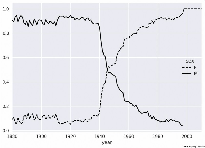
Last , You can easily draw an annual curve by sex ( Pictured 2-10 Shown ):
In [153]: table.plot(style={
'M': 'k-', 'F': 'k--'})
USDA (USDA) A database of information about food nutrition has been made .Ashley Williams Made the data JSON edition (http://ashleyw.co.uk/project/food-nutrient-database). The records are as follows :
{

"id": 21441,
"description": "KENTUCKY FRIED CHICKEN, Fried Chicken, EXTRA CRISPY,
Wing, meat and skin with breading",
"tags": ["KFC"],
"manufacturer": "Kentucky Fried Chicken",
"group": "Fast Foods",
"portions": [
{

"amount": 1,
"unit": "wing, with skin",
"grams": 68.0
},
...
],
"nutrients": [
{

"value": 20.8,
"units": "g",
"description": "Protein",
"group": "Composition"
},
...
]
}
Each food has several identifying attributes and two lists of nutrients and quantities . This form of data is not very suitable for analysis , So we need to do some regularization to make it have a better form .
After downloading and decompressing the data from the URL listed above , You can use whatever you like JSON The library loads it into Python in . I use it Python Built in json modular :
In [154]: import json
In [155]: db = json.load(open('datasets/usda_food/database.json'))
In [156]: len(db)
Out[156]: 6636
db Each entry in is a dictionary that contains all the data about a certain food .nutrients A field is a list of dictionaries , Each of these dictionaries corresponds to a nutrient :
In [157]: db[0].keys()
Out[157]: dict_keys(['id', 'description', 'tags', 'manufacturer', 'group', 'porti
ons', 'nutrients'])
In [158]: db[0]['nutrients'][0]
Out[158]:
{
'description': 'Protein',
'group': 'Composition',
'units': 'g',
'value': 25.18}
In [159]: nutrients = pd.DataFrame(db[0]['nutrients'])
In [160]: nutrients[:7]
Out[160]:
description group units value
0 Protein Composition g 25.18
1 Total lipid (fat) Composition g 29.20
2 Carbohydrate, by difference Composition g 3.06
3 Ash Other g 3.28
4 Energy Energy kcal 376.00
5 Water Composition g 39.28
6 Energy Energy kJ 1573.00
Converting the dictionary list to DataFrame when , You can extract only some of these fields . here , We will take out the name of the food 、 classification 、 Number, manufacturer, etc :
In [161]: info_keys = ['description', 'group', 'id', 'manufacturer']
In [162]: info = pd.DataFrame(db, columns=info_keys)
In [163]: info[:5]
Out[163]:
description group id \
0 Cheese, caraway Dairy and Egg Products 1008
1 Cheese, cheddar Dairy and Egg Products 1009
2 Cheese, edam Dairy and Egg Products 1018
3 Cheese, feta Dairy and Egg Products 1019
4 Cheese, mozzarella, part skim milk Dairy and Egg Products 1028
manufacturer
0
1
2
3
4
In [164]: info.info()
<class 'pandas.core.frame.DataFrame'>
RangeIndex: 6636 entries, 0 to 6635
Data columns (total 4 columns):
description 6636 non-null object
group 6636 non-null object
id 6636 non-null int64
manufacturer 5195 non-null object
dtypes: int64(1), object(3)
memory usage: 207.5+ KB
adopt value_counts, You can check the distribution of food categories :
In [165]: pd.value_counts(info.group)[:10]
Out[165]:
Vegetables and Vegetable Products 812
Beef Products 618
Baked Products 496
Breakfast Cereals 403
Fast Foods 365
Legumes and Legume Products 365
Lamb, Veal, and Game Products 345
Sweets 341
Pork Products 328
Fruits and Fruit Juices 328
Name: group, dtype: int64
Now? , In order to do some analysis of all nutritional data , The simplest way is to integrate the nutrients of all foods into a large table . We do this in several steps . First , Convert the list of nutrients of each food into a DataFrame, And add a column representing the number , Then the DataFrame Add to a list . Finally through concat Just connect these things :
Smooth words ,nutrients The result is :
In [167]: nutrients
Out[167]:
description group units value id
0 Protein Composition g 25.180 1008
1 Total lipid (fat) Composition g 29.200 1008
2 Carbohydrate, by difference Composition g 3.060 1008
3 Ash Other g 3.280 1008
4 Energy Energy kcal 376.000 1008
... ... ...
... ... ...
389350 Vitamin B-12, added Vitamins mcg 0.000 43546
389351 Cholesterol Other mg 0.000 43546
389352 Fatty acids, total saturated Other g 0.072 43546
389353 Fatty acids, total monounsaturated Other g 0.028 43546
389354 Fatty acids, total polyunsaturated Other g 0.041 43546
[389355 rows x 5 columns]
I found this DataFrame In any case, there will be some duplicates , So just throw it away :
In [168]: nutrients.duplicated().sum() # number of duplicates
Out[168]: 14179
In [169]: nutrients = nutrients.drop_duplicates()
Because of two DataFrame All of the objects have "group" and "description", So in order to know who is who , We need to rename them :
In [170]: col_mapping = {
'description' : 'food',
.....: 'group' : 'fgroup'}
In [171]: info = info.rename(columns=col_mapping, copy=False)
In [172]: info.info()
<class 'pandas.core.frame.DataFrame'>
RangeIndex: 6636 entries, 0 to 6635
Data columns (total 4 columns):
food 6636 non-null object
fgroup 6636 non-null object
id 6636 non-null int64
manufacturer 5195 non-null object
dtypes: int64(1), object(3)
memory usage: 207.5+ KB
In [173]: col_mapping = {
'description' : 'nutrient',
.....: 'group' : 'nutgroup'}
In [174]: nutrients = nutrients.rename(columns=col_mapping, copy=False)
In [175]: nutrients
Out[175]:
nutrient nutgroup units value id
0 Protein Composition g 25.180 1008
1 Total lipid (fat) Composition g 29.200 1008
2 Carbohydrate, by difference Composition g 3.060 1008
3 Ash Other g 3.280 1008
4 Energy Energy kcal 376.000 1008
... ... ... ... ... ...
389350 Vitamin B-12, added Vitamins mcg 0.000 43546
389351 Cholesterol Other mg 0.000 43546
389352 Fatty acids, total saturated Other g 0.072 43546
389353 Fatty acids, total monounsaturated Other g 0.028 43546
389354 Fatty acids, total polyunsaturated Other g 0.041 43546
[375176 rows x 5 columns]
To finish these , It can be info Follow nutrients combined :
In [176]: ndata = pd.merge(nutrients, info, on='id', how='outer')
In [177]: ndata.info()
<class 'pandas.core.frame.DataFrame'>
Int64Index: 375176 entries, 0 to 375175
Data columns (total 8 columns):
nutrient 375176 non-null object
nutgroup 375176 non-null object
units 375176 non-null object
value 375176 non-null float64
id 375176 non-null int64
food 375176 non-null object
fgroup 375176 non-null object
manufacturer 293054 non-null object
dtypes: float64(1), int64(1), object(6)
memory usage: 25.8+ MB
In [178]: ndata.iloc[30000]
Out[178]:
nutrient Glycine
nutgroup Amino Acids
units g
value 0.04
id 6158
food Soup, tomato bisque, canned, condensed
fgroup Soups, Sauces, and Gravies
manufacturer
Name: 30000, dtype: object
We can now draw a median map according to food classification and nutrition type ( Pictured 14-11 Shown ):
In [180]: result = ndata.groupby(['nutrient', 'fgroup'])['value'].quantile(0.5)
In [181]: result['Zinc, Zn'].sort_values().plot(kind='barh')

Just use your head a little , You can find out what is the most nutritious food :
by_nutrient = ndata.groupby(['nutgroup', 'nutrient'])
get_maximum = lambda x: x.loc[x.value.idxmax()]
get_minimum = lambda x: x.loc[x.value.idxmin()]
max_foods = by_nutrient.apply(get_maximum)[['value', 'food']]
# make the food a little smaller
max_foods.food = max_foods.food.str[:50]
Because of the DataFrame It's big , So it's not convenient to print all of them in the book . Here only "Amino Acids" Nutrition group :
In [183]: max_foods.loc['Amino Acids']['food']
Out[183]:
nutrient
Alanine Gelatins, dry powder, unsweetened
Arginine Seeds, sesame flour, low-fat
Aspartic acid Soy protein isolate
Cystine Seeds, cottonseed flour, low fat (glandless)
Glutamic acid Soy protein isolate
...
Serine Soy protein isolate, PROTEIN TECHNOLOGIES INTE...
Threonine Soy protein isolate, PROTEIN TECHNOLOGIES INTE...
Tryptophan Sea lion, Steller, meat with fat (Alaska Native)
Tyrosine Soy protein isolate, PROTEIN TECHNOLOGIES INTE...
Valine Soy protein isolate, PROTEIN TECHNOLOGIES INTE...
Name: food, Length: 19, dtype: object
The Federal Election Commission released data on political campaign sponsorship . This includes the name of the sponsor 、 occupation 、 employer 、 Information such as address and capital contribution . We are right. 2012 The data set of the U.S. presidential election in (http://www.fec.gov/disclosurep/PDownload.do). I am here 2012 year 6 The data set downloaded in January is a 150MB Of CSV file (P00000001-ALL.csv), We use first pandas.read_csv Load it in :
In [184]: fec = pd.read_csv('datasets/fec/P00000001-ALL.csv')
In [185]: fec.info()
<class 'pandas.core.frame.DataFrame'>
RangeIndex: 1001731 entries, 0 to 1001730
Data columns (total 16 columns):
cmte_id 1001731 non-null object
cand_id 1001731 non-null object
cand_nm 1001731 non-null object
contbr_nm 1001731 non-null object
contbr_city 1001712 non-null object
contbr_st 1001727 non-null object
contbr_zip 1001620 non-null object
contbr_employer 988002 non-null object
contbr_occupation 993301 non-null object
contb_receipt_amt 1001731 non-null float64
contb_receipt_dt 1001731 non-null object
receipt_desc 14166 non-null object
memo_cd 92482 non-null object
memo_text 97770 non-null object
form_tp 1001731 non-null object
file_num 1001731 non-null int64
dtypes: float64(1), int64(1), object(14)
memory usage: 122.3+ MB
The DataFrame The records in are as follows :
In [186]: fec.iloc[123456]
Out[186]:
cmte_id C00431445
cand_id P80003338
cand_nm Obama, Barack
contbr_nm ELLMAN, IRA
contbr_city TEMPE
...
receipt_desc NaN
memo_cd NaN
memo_text NaN
form_tp SA17A
file_num 772372
Name: 123456, Length: 16, dtype: object
You may have come up with many ways to extract statistics about sponsors and sponsorship patterns from these campaign sponsorship data . I will introduce several different analytical work in the following content ( Apply what you have learned so far ).
It's not hard to see. , There is no party information in this data , So it's better to add it . adopt unique, You can get all the candidate lists :
In [187]: unique_cands = fec.cand_nm.unique()
In [188]: unique_cands
Out[188]:
array(['Bachmann, Michelle', 'Romney, Mitt', 'Obama, Barack',
"Roemer, Charles E. 'Buddy' III", 'Pawlenty, Timothy',
'Johnson, Gary Earl', 'Paul, Ron', 'Santorum, Rick', 'Cain, Herman',
'Gingrich, Newt', 'McCotter, Thaddeus G', 'Huntsman, Jon',
'Perry, Rick'], dtype=object)
In [189]: unique_cands[2]
Out[189]: 'Obama, Barack'
One way to point out party information is to use a dictionary :
parties = {
'Bachmann, Michelle': 'Republican',
'Cain, Herman': 'Republican',
'Gingrich, Newt': 'Republican',
'Huntsman, Jon': 'Republican',
'Johnson, Gary Earl': 'Republican',
'McCotter, Thaddeus G': 'Republican',
'Obama, Barack': 'Democrat',
'Paul, Ron': 'Republican',
'Pawlenty, Timothy': 'Republican',
'Perry, Rick': 'Republican',
"Roemer, Charles E. 'Buddy' III": 'Republican',
'Romney, Mitt': 'Republican',
'Santorum, Rick': 'Republican'}
Now? , Through this mapping and Series Object's map Method , You can get a set of party information based on the candidate's name :
In [191]: fec.cand_nm[123456:123461]
Out[191]:
123456 Obama, Barack
123457 Obama, Barack
123458 Obama, Barack
123459 Obama, Barack
123460 Obama, Barack
Name: cand_nm, dtype: object
In [192]: fec.cand_nm[123456:123461].map(parties)
Out[192]:
123456 Democrat
123457 Democrat
123458 Democrat
123459 Democrat
123460 Democrat
Name: cand_nm, dtype: object
# Add it as a column
In [193]: fec['party'] = fec.cand_nm.map(parties)
In [194]: fec['party'].value_counts()
Out[194]:
Democrat 593746
Republican 407985
Name: party, dtype: int64
Here are two things to pay attention to . First of all , This data includes both sponsorships and refunds ( Negative capital contribution ):
In [195]: (fec.contb_receipt_amt > 0).value_counts()
Out[195]:
True 991475
False 10256
Name: contb_receipt_amt, dtype: int64
To simplify the analysis process , I limit this dataset to positive contributions :
In [196]: fec = fec[fec.contb_receipt_amt > 0]
because Barack Obama and Mitt Romney Are the two main candidates , So I also specially prepared a subset , Only the sponsorship information for the campaign of the two of them :
In [197]: fec_mrbo = fec[fec.cand_nm.isin(['Obama, Barack','Romney, Mitt'])]
Career based sponsorship statistics is another statistical task that is often studied . for example , Lawyers are more inclined to fund Democrats , Business owners, on the other hand, tend to fund the Republican Party . You can't believe me , Just look at the data yourself . First , Calculate the total contribution according to occupation , It's very simple :
In [198]: fec.contbr_occupation.value_counts()[:10]
Out[198]:
RETIRED 233990
INFORMATION REQUESTED 35107
ATTORNEY 34286
HOMEMAKER 29931
PHYSICIAN 23432
INFORMATION REQUESTED PER BEST EFFORTS 21138
ENGINEER 14334
TEACHER 13990
CONSULTANT 13273
PROFESSOR 12555
Name: contbr_occupation, dtype: int64
It's not hard to see. , Many occupations involve the same basic types of work , Or there are many variations of the same thing . The following code snippet can clean up some of this data ( Map one career information to another ). Be careful , Here is a clever use of dict.get, It allows classes that do not have a mapping relationship to “ adopt ”:
occ_mapping = {

'INFORMATION REQUESTED PER BEST EFFORTS' : 'NOT PROVIDED',
'INFORMATION REQUESTED' : 'NOT PROVIDED',
'INFORMATION REQUESTED (BEST EFFORTS)' : 'NOT PROVIDED',
'C.E.O.': 'CEO'
}
# If no mapping provided, return x
f = lambda x: occ_mapping.get(x, x)
fec.contbr_occupation = fec.contbr_occupation.map(f)
I did the same with the employer information :
emp_mapping = {

'INFORMATION REQUESTED PER BEST EFFORTS' : 'NOT PROVIDED',
'INFORMATION REQUESTED' : 'NOT PROVIDED',
'SELF' : 'SELF-EMPLOYED',
'SELF EMPLOYED' : 'SELF-EMPLOYED',
}
# If no mapping provided, return x
f = lambda x: emp_mapping.get(x, x)
fec.contbr_employer = fec.contbr_employer.map(f)
Now? , You can go through pivot_table Aggregate data by Party and occupation , Then filter out the insufficient total contribution 200 Million dollars :
In [201]: by_occupation = fec.pivot_table('contb_receipt_amt',
.....: index='contbr_occupation',
.....: columns='party', aggfunc='sum')
In [202]: over_2mm = by_occupation[by_occupation.sum(1) > 2000000]
In [203]: over_2mm
Out[203]:
party Democrat Republican
contbr_occupation
ATTORNEY 11141982.97 7.477194e+06
CEO 2074974.79 4.211041e+06
CONSULTANT 2459912.71 2.544725e+06
ENGINEER 951525.55 1.818374e+06
EXECUTIVE 1355161.05 4.138850e+06
... ... ...
PRESIDENT 1878509.95 4.720924e+06
PROFESSOR 2165071.08 2.967027e+05
REAL ESTATE 528902.09 1.625902e+06
RETIRED 25305116.38 2.356124e+07
SELF-EMPLOYED 672393.40 1.640253e+06
[17 rows x 2 columns]
It will be clearer to make these data into a histogram ('barh’ Represents a horizontal bar graph , Pictured 14-12 Shown ):
In [205]: over_2mm.plot(kind='barh')

You may also want to know about Obama and Romney The occupation and enterprise with the highest total capital contribution . So , Let's group the candidates first , Then use something similar to the one described earlier in this chapter top Methods :
def get_top_amounts(group, key, n=5):
totals = group.groupby(key)['contb_receipt_amt'].sum()
return totals.nlargest(n)
Then aggregate according to occupation and employer :
In [207]: grouped = fec_mrbo.groupby('cand_nm')
In [208]: grouped.apply(get_top_amounts, 'contbr_occupation', n=7)
Out[208]:
cand_nm contbr_occupation
Obama, Barack RETIRED 25305116.38
ATTORNEY 11141982.97
INFORMATION REQUESTED 4866973.96
HOMEMAKER 4248875.80
PHYSICIAN 3735124.94
...
Romney, Mitt HOMEMAKER 8147446.22
ATTORNEY 5364718.82
PRESIDENT 2491244.89
EXECUTIVE 2300947.03
C.E.O. 1968386.11
Name: contb_receipt_amt, Length: 14, dtype: float64
In [209]: grouped.apply(get_top_amounts, 'contbr_employer', n=10)
Out[209]:
cand_nm contbr_employer
Obama, Barack RETIRED 22694358.85
SELF-EMPLOYED 17080985.96
NOT EMPLOYED 8586308.70
INFORMATION REQUESTED 5053480.37
HOMEMAKER 2605408.54
...
Romney, Mitt CREDIT SUISSE 281150.00
MORGAN STANLEY 267266.00
GOLDMAN SACH & CO. 238250.00
BARCLAYS CAPITAL 162750.00
H.I.G. CAPITAL 139500.00
Name: contb_receipt_amt, Length: 20, dtype: float64
You can also do another very practical analysis of the data : utilize cut The function discretizes the data into multiple facets according to the size of the contribution :
In [210]: bins = np.array([0, 1, 10, 100, 1000, 10000,
.....: 100000, 1000000, 10000000])
In [211]: labels = pd.cut(fec_mrbo.contb_receipt_amt, bins)
In [212]: labels
Out[212]:
411 (10, 100]
412 (100, 1000]
413 (100, 1000]
414 (10, 100]
415 (10, 100]
...
701381 (10, 100]
701382 (100, 1000]
701383 (1, 10]
701384 (10, 100]
701385 (100, 1000]
Name: contb_receipt_amt, Length: 694282, dtype: category
Categories (8, interval[int64]): [(0, 1] < (1, 10] < (10, 100] < (100, 1000] < (1
000, 10000] <
(10000, 100000] < (100000, 1000000] < (1000000,
10000000]]
Obama and Romney data can now be grouped by candidate names and bin tags , To get a histogram :
In [213]: grouped = fec_mrbo.groupby(['cand_nm', labels])
In [214]: grouped.size().unstack(0)
Out[214]:
cand_nm Obama, Barack Romney, Mitt
contb_receipt_amt
(0, 1] 493.0 77.0
(1, 10] 40070.0 3681.0
(10, 100] 372280.0 31853.0
(100, 1000] 153991.0 43357.0
(1000, 10000] 22284.0 26186.0
(10000, 100000] 2.0 1.0
(100000, 1000000] 3.0 NaN
(1000000, 10000000] 4.0 NaN
From this data, we can see , In the area of small sponsorship ,Obama The quantity obtained is more than Romney A lot more . You can also sum the contributions and normalize them in the bin , So as to graphically display the proportion of various sponsorship amounts of the two candidates ( See the picture 14-13):
In [216]: bucket_sums = grouped.contb_receipt_amt.sum().unstack(0)
In [217]: normed_sums = bucket_sums.div(bucket_sums.sum(axis=1), axis=0)
In [218]: normed_sums
Out[218]:
cand_nm Obama, Barack Romney, Mitt
contb_receipt_amt
(0, 1] 0.805182 0.194818
(1, 10] 0.918767 0.081233
(10, 100] 0.910769 0.089231
(100, 1000] 0.710176 0.289824
(1000, 10000] 0.447326 0.552674
(10000, 100000] 0.823120 0.176880
(100000, 1000000] 1.000000 NaN
(1000000, 10000000] 1.000000 NaN
In [219]: normed_sums[:-2].plot(kind='barh')
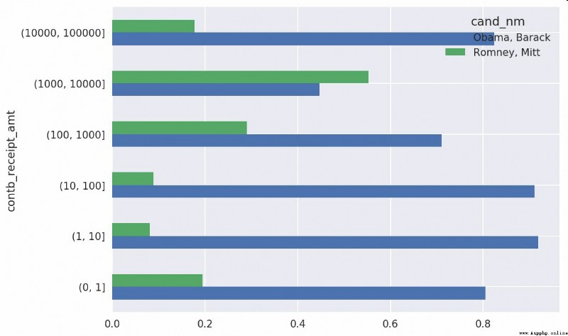
I excluded the two largest facets , Because these are not donated by individuals .
The analysis process can also be refined and improved . for instance , The data can be aggregated according to the sponsor's name and postal code , To find out who made multiple small donations , Who has made one or more large donations . I strongly recommend that you download the data and try it yourself .
Aggregating data by candidate and state is a common practice :
In [220]: grouped = fec_mrbo.groupby(['cand_nm', 'contbr_st'])
In [221]: totals = grouped.contb_receipt_amt.sum().unstack(0).fillna(0)
In [222]: totals = totals[totals.sum(1) > 100000]
In [223]: totals[:10]
Out[223]:
cand_nm Obama, Barack Romney, Mitt
contbr_st
AK 281840.15 86204.24
AL 543123.48 527303.51
AR 359247.28 105556.00
AZ 1506476.98 1888436.23
CA 23824984.24 11237636.60
CO 2132429.49 1506714.12
CT 2068291.26 3499475.45
DC 4373538.80 1025137.50
DE 336669.14 82712.00
FL 7318178.58 8338458.81
If you divide each line by the total sponsorship , You will get the proportion of the total sponsorship of each candidate in each state :
In [224]: percent = totals.div(totals.sum(1), axis=0)
In [225]: percent[:10]
Out[225]:
cand_nm Obama, Barack Romney, Mitt
contbr_st
AK 0.765778 0.234222
AL 0.507390 0.492610
AR 0.772902 0.227098
AZ 0.443745 0.556255
CA 0.679498 0.320502
CO 0.585970 0.414030
CT 0.371476 0.628524
DC 0.810113 0.189887
DE 0.802776 0.197224
FL 0.467417 0.532583
#14.6 summary
We have completed the last chapter of the text . There are some additional contents in the appendix , May be useful to you .
The first edition of this book has been published for 5 Years. ,Python Has become a popular 、 A widely used data analysis language . What you learned from this book , It is available for a long time . I hope the tools and libraries introduced in this book will be useful for your work .
 Imageai continued deepstack (II) fast and simple object detection using Python
One . brief introduction DeepS
 Python crawler Baidu translator, the code is OK, sometimes the operation is OK, and the following error is reported
{error_code: 54003, error_msg: