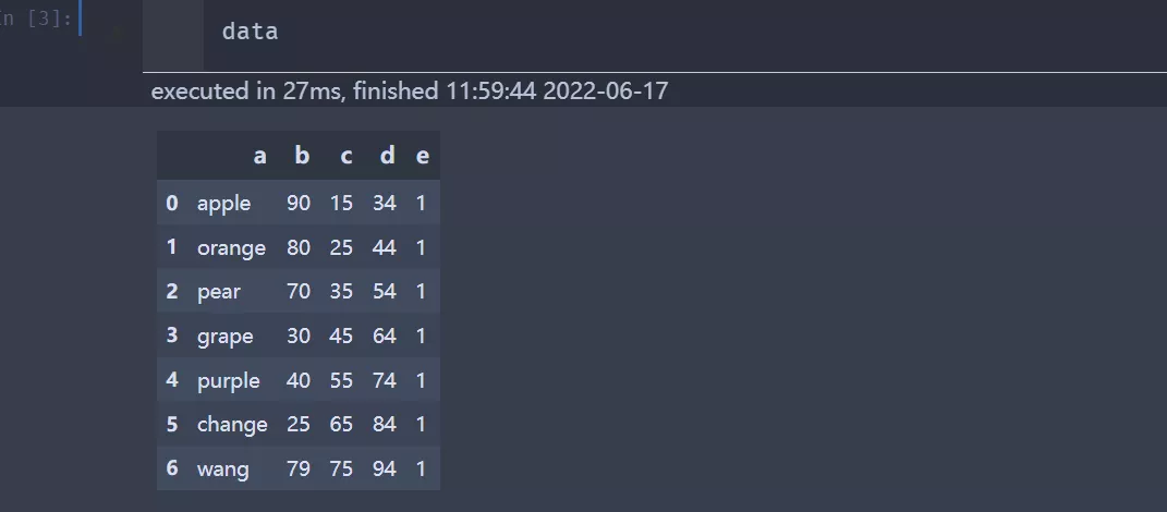
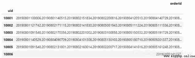
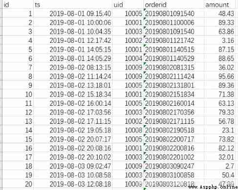
The data field contains : Self increasing id, The order time ts, user id, Order id, Order amount 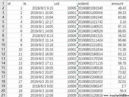
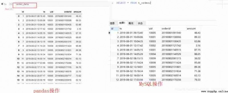
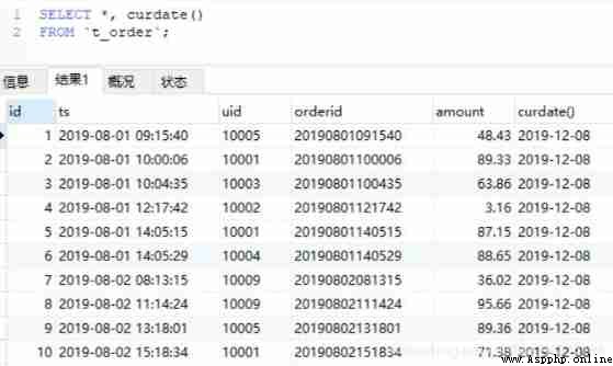
Look at all the data ,pandas Print directly in dataframe Object can , Here is order_data. And in the SQL in , The statement to be executed is select * from t_order; From t_order Query all the data in the table ,* Sign means to query all fields
#python
import pandas as pd
order_data = pd.read_csv('order.csv')
order_data # View all data
order_data.head(10) # See the former 10 That's ok
#MySQL
select * from t_order; # View all data
select * from t_order limit 10; # See the former 10 That's ok
If you just want to view the front 10 What about row data .pandas You can call head(n) Method ,n It's the number of lines .MySQL have access to limit n,n It also represents the number of rows 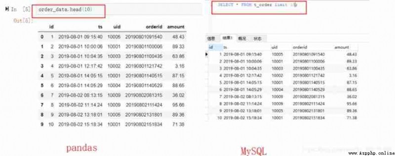
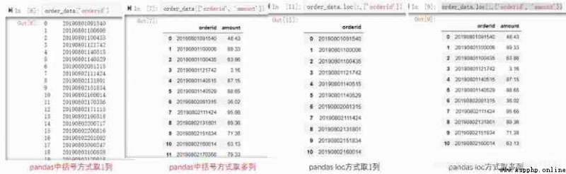
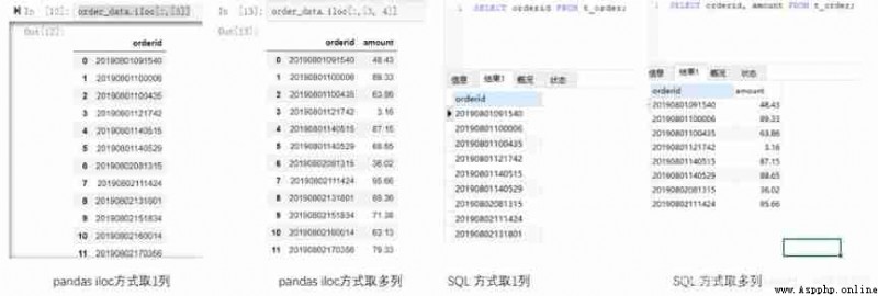
stay pandas You can use brackets or loc,iloc And so on , You can select one or more columns .loc You can write column names directly ,iloc The method needs to specify the index , Which column .SQL Just write the corresponding column name in the
#Python
order_data['orderid'] # View the specified column
order_data.loc[:,['orderid']] # View the specified column
order_data.iloc[:,[3]] # View the specified column
order_data[['orderid', 'amount']] # View the specified columns
order_data.loc[:,['orderid', 'amount']] # View the specified columns
order_data.iloc[:,[3, 4]] # View the specified columns
#MySQL
select orderid from t_order; # View the specified column
select orderid, amount from t_order; # View the specified columns
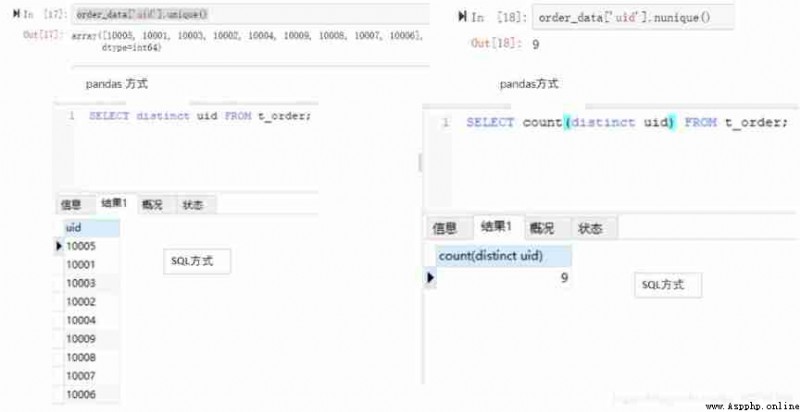
See how many people there are ( Get rid of the heavy ones ) I've ordered .pandas Are there in unique Method ,SQL Are there in distinct keyword . As shown in the code on the left side of the figure below . The output of both methods contains 9 individual uid, And know where it is 9 individual . If you just want to know how many uid, If you don't pay attention to specific values , You can refer to the... On the right SQL,pandas use nunique() Method realization , and SQL You need one in the count Aggregate function and distinct The way of combination , Means to remove the weight and count .
#Python
order_data['uid'].unique() # duplicate removal
order_data['uid'].nunique() # To count again
#MySQL
select distinct uid from t_order; # duplicate removal
select count(distinct uid) from t_order; # To count again
1) belt 1 Conditions
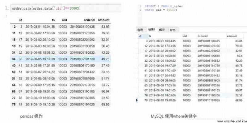
For example, we need to check uid by 10003 All records .pandas You need to use a Boolean index , and SQL Required in where keyword . When specifying conditions , Equivalent conditions can be specified , Unequal conditions can also be used , Such as greater than or less than . But be sure to pay attention to data types . For example, if uid It's a string type , You need to 10003 Put quotes , This is an integer type, so there is no need to add .
#Python
order_data[order_data['uid']==10003]
#MySQL
select * from t_order where uid=10003;
2) With multiple conditions
Multiple conditions are met at the same time :
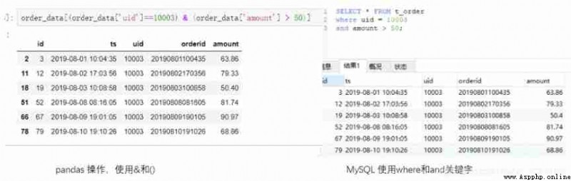
On the basis of the previous summary ,pandas Need to use & Symbols connect multiple conditions , Each condition needs to be enclosed in parentheses ;SQL Need to use and Keyword connects multiple conditions . So let's say we query uid by 10003 And the amount is greater than 50 The record of .
#Python
order_data[(order_data['uid']==10003) & (order_data['amount']>50)]
#MySQL
select * from t_order where uid=10003 and amount>50;
The case where multiple conditions satisfy one of them :
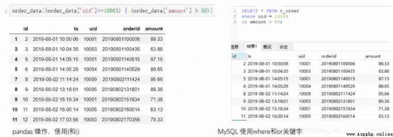
Use when multiple conditions are met at the same time & Corresponding , We use | The symbol denotes a condition that is satisfied , and SQL In the middle, we use or Keyword connects each condition to indicate that any one is satisfied .
#Python
order_data[(order_data['uid']==10003) | (order_data['amount']>50)]
#MySQL
select * from t_order where uid=10003 or amount>50;
It should be noted here that there is a case where you need to judge whether a field is null .pandas For null value of nan Express , The judgment conditions need to be written as isna(), perhaps notna().
#Python
# lookup uid Not empty record
order_data[order_data['uid'].notna()]
# lookup uid Empty record
order_data[order_data['uid'].isna()]
MySQL The corresponding judgment statement needs to be written as is null perhaps is not null.
#MySQL
select * from t_order where uid is not null;
select * from t_order where uid is null;
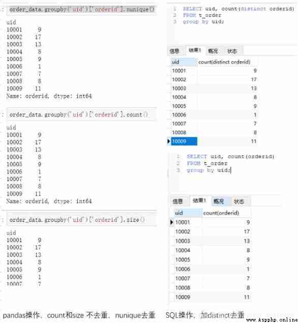
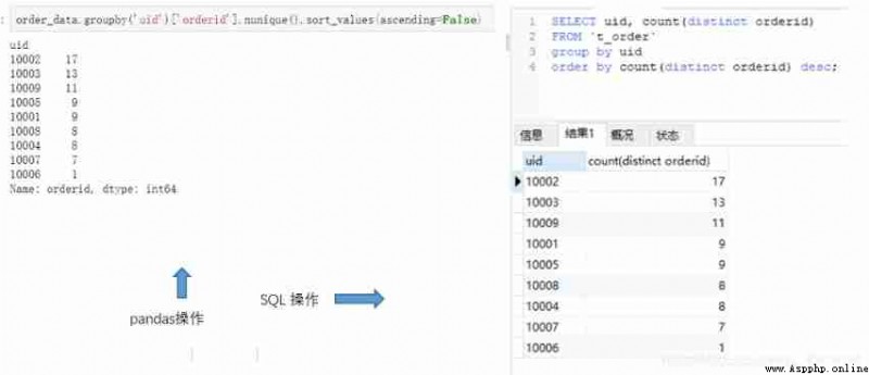
Use groupby when , This is usually accompanied by an aggregation operation , In this case, you need to use the aggregate function . aforementioned count Is an aggregate function , To count , Besides, there is sum It means sum ,max,min Indicates the maximum and minimum value, etc .pandas and SQL Both support aggregation operations . For example, we ask each uid How many orders are there
#Python
order_data.groupby('uid')['orderid'].nunique() # Count the non repeated numbers in groups ( duplicate removal )
order_data.groupby('uid')['orderid'].count() # Group count ( Contains the number of duplicates )( No weight removal )
order_data.groupby('uid')['orderid'].size() # Group count ( Contains the number of duplicates )( No weight removal )
#MySQL
select uid, count(distinct orderid) from t_order group by uid; # duplicate removal
select uid, count(orderid) from t_order group by uid; # No weight removal
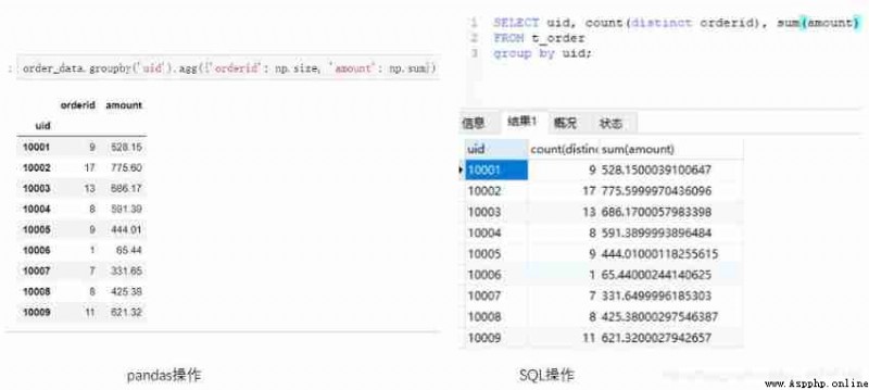
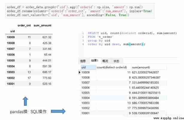
If you want to perform different aggregation operations on different fields at the same time . For example, the goal becomes : Please, everyone uid Order quantity and total order amount .
#Python
order_data.groupby('uid').agg({
'order_id':np.size, 'amount':np.sum})
#MySQL
select uid, count(distinct orderid), sum(amount) from t_order group by uid;
further , We can rename the resulting dataset .pandas have access to rename Method ,MySQL have access to as Keyword to rename the result .
#Python
order_df=order_data.groupby('uid').agg({
'order_id':np.size, 'amount':np.sum})
order_df.rename(columns={
'order_id':'order_cnt', 'amount':'sum_amount'})
#MySQL
select uid, count(distinct orderid) as order_cnt, sum(amount) as sum_amount from t_order group by uid;

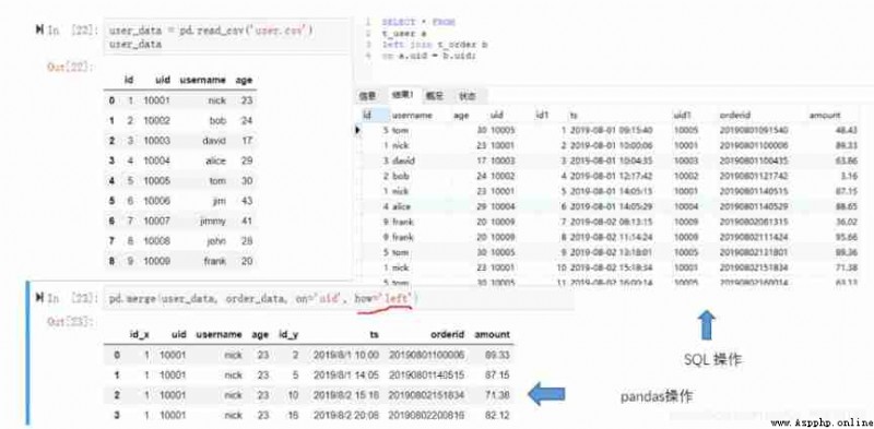
join Related operations are inner join,left join,right join,full join, etc. .pandas China unified through pd.merge Method , Setting different parameters can achieve different dataframe The connection of . and SQL You can directly use the corresponding keywords to connect the two tables . To demonstrate , Here we introduce a new dataset ,user.csv( Corresponding to t_user surface ). Contains the user's nickname , Age information .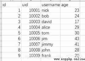
1) left join
pandas Of merge Function is introduced to 4 Parameters , The first is the connected main table , The second is to join the slave table , The third connected key value , The fourth is the way of connection ,how by left Time means left connection .SQL The operation is basically the same logic , To specify the main table , From the table , Connection mode and connection field . Here we use user Connect order And query all fields and all records . The specific code is as follows , Because our data has no null value , Therefore, it does not reflect the characteristics of left connection .
#Python
user_data = pd.read_csv('user.csv')
pd.merge(user_data, order_data, on='uid', how='left')
#MySQL
select * from t_user a left join t_order b on a.uid=b.uid;
2) Other connections
If we want to achieve inner join,outer join,right join,pandas Corresponding how Parameter is inner( Default ),outer,right.SQL You can also directly use the corresponding keywords . among inner join Can be abbreviated to join.
#Python
pd.merge(user_data, order_data, on='uid', how='inner')
#MySQL
SELECT * FROM
t_user a
inner join t_order b
on a.uid = b.uid;
union Related operations are divided into union and union all Two kinds of . They are usually used in scenarios where two pieces of data with the same field are vertically spliced together . But the former will be de duplicated . for example , I have one now order2 Order data for , Included fields and order The data is consistent , I want to merge the two into one dataframe in .SQL In this scenario, it is also expected that order2 Table and order Table merge output .
#Python
order_union=pd.concat([order_data, order_data2])
order_union
#MySQL
select * from
t_order
union all
select * from
t_order2;
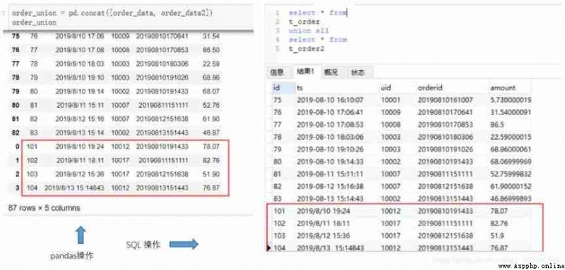
The above is the case without weight removal , If you want to go heavy ,SQL Need to use union keyword . and pandas You need to add a redo operation .
#Python
order_union = pd.concat([order_data, order_data2]).drop_duplicates()
#MySQL
select * from
t_order
union
select * from
t_order2;
In practical work, it is often necessary to sort by a certain column of fields .pandas Sorting in uses sort_values Method ,SQL Sorting in can use order_by keyword . We use an example to illustrate : According to each uid The number of orders is sorted from high to low . This is based on the previous aggregation operation
#Python
order_data.groupby('uid')['orderid'].nunique().sort_values(ascending=False)
#MySQL
select uid, count(distinct orderid) from t_order
group by uid
order by count(distinct orderid) desc;
Sorting time ,asc Expressing ascending order ,desc Representation of descending order , You can see that both methods specify the sort method , The reason is that by default, they are arranged in ascending order . On this basis , You can sort multiple fields .pandas in ,dataframe For multi field sorting, you need to use by Specify sort fields ,SQL Just write multiple fields in order order by After that . for example , Output uid, Number of orders , The order amount is listed in three columns , And in accordance with the uid Descending , The order amount is arranged in ascending order .
#Python
order_df=order_data.groupby('uid').agg({
'order_id':np.size, 'amount':np.sum})
order_df.rename(columns={
'orderid':'order_cnt','amount':'sum_amount'}, inplace=True)
order_df.sort_values(by=['uid', 'sum_amount'], ascending=[False, True])
stay pandas There may be some details to pay attention to , For example, we assign values to the aggregation results first , Then rename , And designated inplace=True Replace the original name , Then sort , Although it is a bit convoluted , But the overall thinking is relatively clear .
#MySQL
select uid, count(distinct orderid),sum(amount) from t_order
group by uid
order by uid desc, sum(amount);
Compared to other operations ,case when The operation may not be so “ Universal ”. It is more common in SQL Scene , May be used for grouping , May be used for assignment , It can also be used in other scenarios . grouping , For example, it is divided into good, medium and poor according to a certain score range . assignment , For example, when the value is less than 0 when , according to 0 Calculation . Let's take a group scenario for example . Each one uid Divided into... According to the total amount [0-300),[300,600),[600,900) Three groups of .
#Python
def func(x):
if x<300:
return '[0-300)'
elif x<600:
return '[300-600)'
else:
return '[600-900)'
order_df['amt_interval']=order_df['sum_amount'].map(func)
order_df
#MySQL
select uid, order_cnt,
case when sum_amount<300 then '[0-300)'
when sum_amount>=300 and sum_amount<600 then '[300-600)'
when sum_amount>=600 and sum_amount<900 then '[600-900)'
else 'other' end as amt_interval
from
(
select uid, count(distinct orderid) order_cnt, sum(amount) as sum_amount
from t_order
group by uid
order by uid desc, sum(amount)
) a
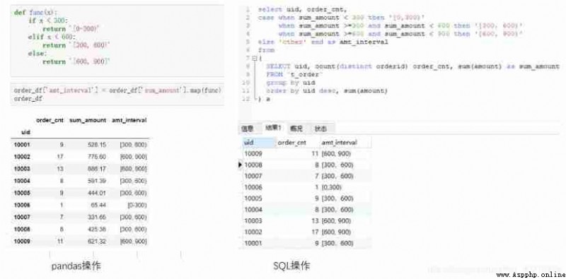
be familiar with pandas My friends should be able to think of ,pandas There is a special term for this grouping operation of “ Separate boxes ”, The corresponding function is cut,qcut, Can achieve the same effect . In order to maintain and SQL Consistency of operations , It is used here map How to function .
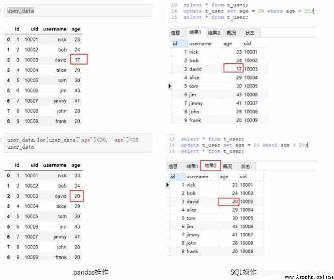
1) to update
Both update and delete are operations to change the original data . For update operations , The logic of the operation is : First select the target row that needs to be updated , Update again .pandas in , You can use the method mentioned above to select , After that, you can directly assign values to the target column ,SQL Required in update Keyword to update the table . Examples are as follows : Will be younger than 20 The user age of is changed to 20.
#Python
user_data
user_data.loc[user_data['age']<20, 'age']=20
user_data
#MySQL
select * from t_user;
update t_user set age=20 where age<20;
select * from t_user;
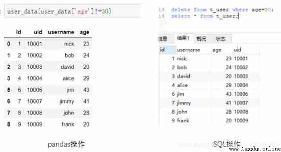
2) Delete
Deletion can be subdivided into row deletion and column deletion . For delete row operation ,pandas The delete line of can be converted to the operation of selecting unqualified lines .SQL Need to use delete keyword . For example, delete the age as 30 Year old user .
#Python
user_data[user_data['age']!=30]
user_data
#MySQL
delete from t_user where age=30;
select * from t_user;
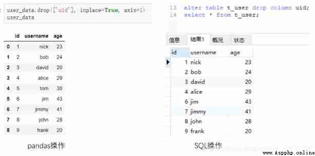
For deleting Columns .pandas Need to use drop Method .SQL Also need to use drop keyword .
#Python
user_data.drop(['uid'], inplace=True, axis=1)
user_data
#MySQL
alter table t_user drop column uid;
select * from t_user;
summary :
hive Aspect we created a new table , And load the same data into the table .
#hive
# Build table
create table t_order(
id int comment "id",
ts string comment ' The order time ',
uid string comment ' user id',
orderid string comment ' Order id',
amount float comment ' Order amount '
)
row format delimited fields terminated by ','
stored as textfile;
# Load data
load data local inpath 'order.csv' overwrite into table t_order;
# Load data
select * from t_order;

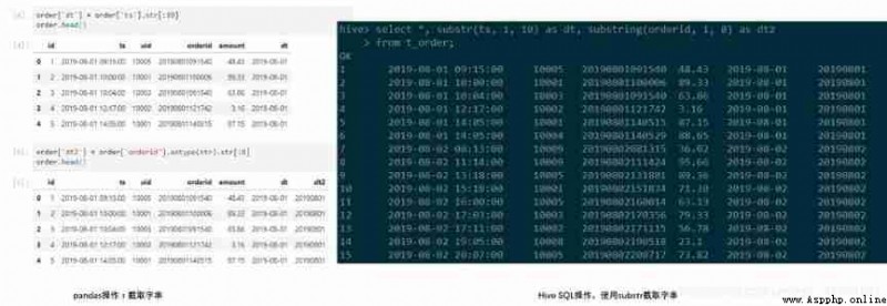
For a column in the original dataset , We often have to intercept its string as a new column to use . For example, we want to find the date corresponding to each order . Need from order time ts perhaps orderid Medium intercept . stay pandas in , We can convert a column to a string , Intercept its substring , Add as new column . We use .str Treat the original field as a string , from ts Before intercepting 10 position , from orderid Before intercepting 8 position . Experience shows that sometimes in .str It needs to be added before astype.
For the operation of string interception ,Hive SQL There is substr function , It's in MySQL and Hive The usage in is the same substr(string A,int start,int len) Represents from string A The starting position of interception in is start, The length is len The string of , Where the starting position is from 1 Start counting .
#python
import pandas as pd
order = pd.read_csv('order.csv', names=['id', 'ts', 'uid', 'orderid', 'amount'])
order.head()
order['dt'] = order['ts'].str[:10]
order.head()
order['dt2'] = order['orderid'].astype(str).str[:8]
order.head()
#Hive SQL
select *, substr(ts, 1, 10) as dt, substr(orderid, 1, 8) as dt2
from t_order;
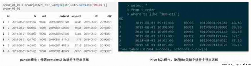
Extract fields that contain specific characters , stay pandas We can use the string in contains,extract,replace Method , regular expression . And in the hive SQL in , There are simple Like Keyword matches a specific character , You can also use regexp_extract,regexp_replace These two functions are more flexible in achieving the goal .
Suppose you want to realize Screening The order time includes “08-01” The order of .pandas and SQL The code is as follows , Use like when ,% The wildcard , Means to match characters of any length .
#python
order_08_01 = order[order['ts'].astype(str).str.contains('08-01')]
order_08_01
#Hive SQL
select * from t_order where ts like "%08-01%";
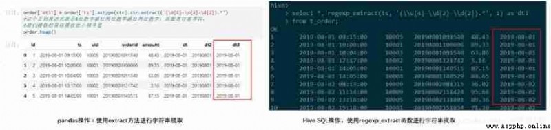
Suppose you want to realize extract ts Date information in ( front 10 position ),pandas Support regular expressions in extract function , and hive In addition to the above mentioned substr Function can be implemented outside , Here we can use regexp_extract function , Through regular expressions .
#python
order['dt3'] = order['ts'].astype(str).str.extract('(\d{4}-\d{2}-\d{2}).*')
# This regular expression represents "4 Two digit horizontal bar two digit horizontal bar two digit ", Followed by any character ,. The wildcard ,* Express 0 Times or times ,
# The target we extract should be placed in parentheses
order.head()
#Hive SQL
select *, regexp_extract(ts, '(\\d{4}-\\d{2}-\\d{2}).*', 1) as dt3
from t_order;
# Our goal is also in parentheses ,1 Means to take the first matching result
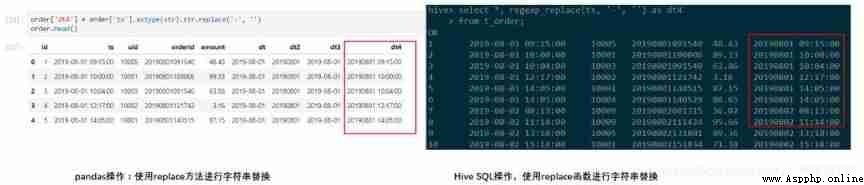
Suppose we want to Get rid of ts The horizontal bar in , That is, replacement ts Medium “-” It's empty , stay pandas String can be used in replace Method ,hive Can be used in regexp_replace function .
#python
order['dt4'] = order['ts'].astype(str).str.replace('-', '')
order.head()
#Hive SQL
select *, regexp_replace(ts, '-', '') as dt4
from t_order;
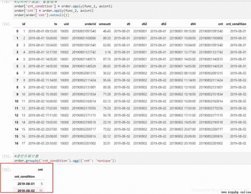
We want to count :ts contains ‘2019-08-01’ How many non repeat orders are there ,ts contains ‘2019-08-02’ How many non repeat orders are there .
#Hive SQL
select count(distinct case when ts like '%2019-08-01%' then orderid end) as 0801_cnt,
count(distinct case when ts like '%2019-08-02%' then orderid end) as 0802_cnt
from t_order;
# Running results :
5 11
pandas To realize :
Define two functions , The first function adds a column to the original data , Mark our conditions , The second function adds another column , When the conditions are met , Give corresponding orderid, And then to the whole dataframe Apply these two functions . For lines we don't care about , The values for both columns are nan. The third step is to perform the operation of de counting .
#python
# First step : Construct an auxiliary column
def func_1(x):
if '2019-08-01' in x['ts']:
return '2019-08-01'# This place can return other tags
elif '2019-08-02' in x['ts']:
return '2019-08-02'
else:
return None
# The second step : Will meet the conditions order As a new column
def func_2(x):
if '2019-08-01' in x['ts']:
return str(x['orderid'])
elif '2019-08-02' in x['ts']:
return str(x['orderid'])
else:
return None
# Apply two functions , View results
# Note that... Must be added here axis=1, You can try what will happen if you don't add it
order['cnt_condition'] = order.apply(func_1, axis=1)
order['cnt'] = order.apply(func_2, axis=1)
order[order['cnt'].notnull()]
# Group count
order.groupby('cnt_condition').agg({
'cnt': 'nunique'})
row_number() over The basic usage of function
grammar :row_number() over (partition by column1 order by column2)
Detailed explanation : according to column1 Grouping , Within the group according to column2 Sort , The value calculated by this function represents the sequence number of each group after internal sorting ( Each group is numbered from 1 Began to increase , The number is continuous and unique within the group ).
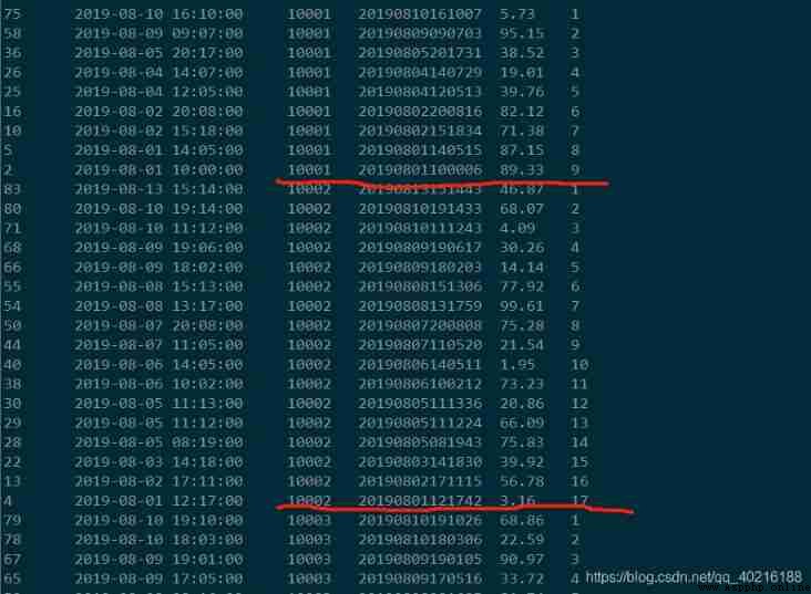
For example, we treat each uid Orders for are arranged in reverse order of order time , Get the sequence number of its sorting .
#pandas We need the help of groupby and rank Function to achieve the same effect .
# change rank Medium method Parameters can be implemented Hive Other sorting in
# Because of our ts Fields are string types , First convert to datetime type
order['ts2'] = pd.to_datetime(order['ts'], format='%Y-%m-%d %H:%M:%S')
# Group sort , according to uid grouping , according to ts2 Descending , The serial number defaults to decimal , Need to convert to an integer
# And add as a new column rk
order['rk'] = order.groupby(['uid'])['ts2'].rank(ascending=False, method='first').astype(int)
# For ease of viewing rk The effect of , For the original data, follow uid And time , Results and SQL Agreement
order.sort_values(['uid','ts'], ascending=[True, False])
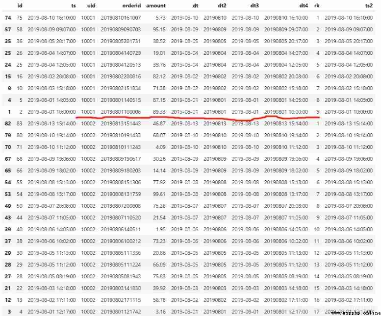
select *, row_number() over (partition by uid order by ts desc) as rk
from t_order;
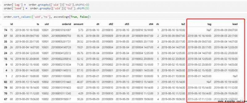
#ag and lead The function is also Hive SQL Window functions commonly used in , Their format is :
lag( Field name ,N) over(partition by Grouping field order by Sort field sort order )
lead( Field name ,N) over(partition by Grouping field order by Sort field sort order )
lag Function representation , It is smaller than the sequence number of this record after grouping and sorting N The value of the specified field of the corresponding record .lead Just the opposite , Is larger than the current record N The specified field value of the corresponding record of
select *,
lag(ts, 1) over (partition by uid order by ts desc) as lag,
lead(ts, 1) over (partition by uid order by ts desc) as lead
from t_order;

In the example lag Indicates that after grouping and sorting , Of the previous record ts,lead Indicates the last record ts. Nonexistent use NULL fill .
pandas We also have corresponding shift Function to implement such a requirement .shift When the parameter of is a positive number , Express lag, When it's negative , Express lead.
order['lag'] = order.groupby(['uid'])['ts2'].shift(-1)
order['lead'] = order.groupby(['uid'])['ts2'].shift(1)
# Still to see the effect , For the original data, follow uid And time , Results and SQL Agreement
order.sort_values(['uid','ts'], ascending=[True, False])
In our data , One uid It will correspond to multiple orders , At present, there are many orders id It is displayed in multiple lines . Now what we need to do is make multiple orders id Show in the same line , Separate... With commas . stay pandas in , What we do is to replace the original orderid Column to string form , And in every id Add a comma as the delimiter at the end , Then use the method of string addition , Each one uid The corresponding string type order id Splicing together . The code and effect are as follows . In order to reduce interference , We will order Data re read , And set up pandas How to display .
#Python
import pandas as pd
pd.set_option('display.max_columns', None) # Show all columns
pd.set_option('display.max_rows', None) # Show all lines
pd.set_option('display.max_colwidth', 100) # The maximum display length of the column is 100
order=pd.read_csv('order.csv', names=['id', 'ts', 'uid', 'orderid', 'amount'])
order.head()

#Python
order['orderid']=order['orderid'].astype('str')
order['orderid']=order['orderid'].apply(lambda x: x+',')
order_group=order.groupby('uid').agg('orderid':'sum')
order_group
You can see , The same uid Corresponding order id Already displayed on the same line , Order id Separated by commas .
stay Hive It is much more convenient to achieve the same effect in , We can use collect_set/collect_list function ,, The difference between the two is that the former will be de duplicated during polymerization , Don't forget to add group by.
#Hive
select uid, collect_set(orderid) as order_list
from t_order group by uid;
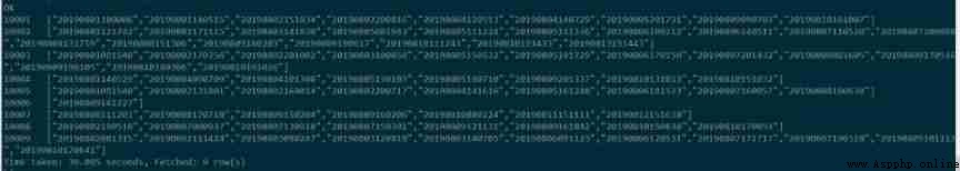
It can be seen that hive In the effect achieved , Will be the same uid Of orderid As a “ Array ” Show it .
UDTF(User-Defined Table-Generating Functions) It is used to solve the demand function of inputting one line and outputting multiple lines .
lateral view Used for and split、explode etc. UDTF Used together , Can split a line of data into multiple lines of data , On this basis, the split data can be aggregated ,lateral view First call... For each row of the original table UDTF,UDTF Will split a row into one or more rows ,lateral view Combining the results , Generate a virtual table that supports alias tables .
grammar : lateral view UDTF(expression) tableAliasName as colAliasName
among UDTF(expression) Is a function of row to column , That is, a function from one line to multiple lines , such as explode.
tableAliasName Represents an alias for a table ,colAliasName An alias that represents a column of a table .
principle : adopt lateral view UDTF(expression) Function to convert a line to multiple lines , A temporary table will be generated , Put this data into this temporary table .
1) Single lateral view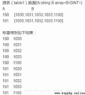
select A,B from table_1 lateral view explode(B) mytable as B;
2) Multiple lateral view
Source table basetable, contain col1 and col2 Two column data , The data sheet is as follows :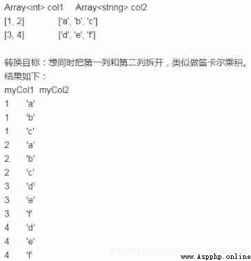
select mycol1, mycol2 from basetable
lateral view explode(col1) mytable1 as mycol1
lateral view explode(col2) mytable2 as mycol2;
3) Complex ways 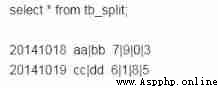
select datenu, des, t from tb_split
lateral view explode(split(des,"\\|")) tb1 as des
lateral view explode(split(t,"\\|")) tb2 as t;
4) Restore the results from the previous section to each orderid Show the form of one line
with tmp as
(
select uid, collect_set(orderid) as order_list
from t_order
group by uid
)
select uid, o_list
from tmp lateral view explode(order_list) t as o_list;
When we write something with relatively complex structure SQL When the sentence is , It is possible that a sub query may be reused in multiple levels and places , We can use it at this time with as Statement to separate it , Greatly improved SQL Readability , simplify SQL~
notes : at present oracle、sql server、hive And so on with as usage , but mysql Does not support !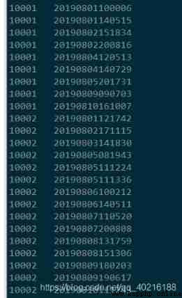
python The implementation is as follows :
order_group = order_group.reset_index() # Reset the index
order_group
order_group1 = pd.concat([pd.Series(row['uid'], row['orderid'].split(',')) for _ , row in order_group.iterrows()]).reset_index()
order_group1
There will be a blank line in the result , This is because when separated by commas , The last element is empty .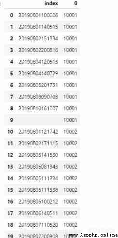
Load new data 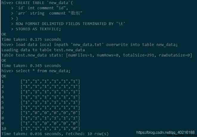
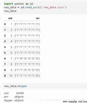
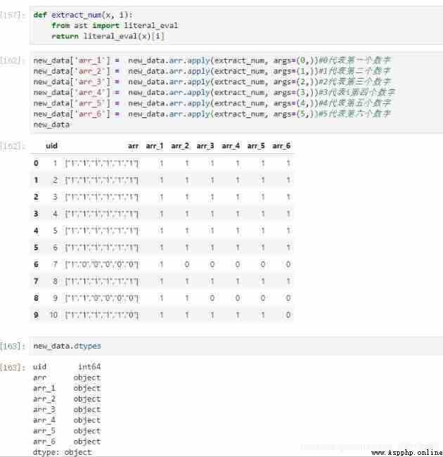
First look pandas To realize , Here we need to use literal_eval This package , Can automatically identify the array stored in the form of string . I defined an analytic function , take arr Column applies the function more than once , The parsed result is treated as a new column :
def extract_num(x, i):
from ast import literal_eval
return literal_eval(x)[i]
new_data['arr_1']=new_data.arr.apply(extract_num, args=(0,)) #0 Represents the first number
new_data['arr_2']=new_data.arr.apply(extract_num, args=(1,)) #1 Represents the second number
new_data['arr_3']=new_data.arr.apply(extract_num, args=(2,)) #2 That's the third number
new_data['arr_4']=new_data.arr.apply(extract_num, args=(3,)) #3 Represents the fourth digit
new_data['arr_5']=new_data.arr.apply(extract_num, args=(4,)) #4 Represents the fifth digit
new_data['arr_6']=new_data.arr.apply(extract_num, args=(5,)) #5 Represents the sixth digit
#new_data['arr_1'] = new_data.arr.apply(extract_num, args=(0,)).astype(int)
# The result of analysis is object Type of , If you want them to participate in numerical calculations , It needs to be converted to int type
new_data
go back to Hive SQL, It's easier to implement . We can go through split Function to change the original string form into an array , Then take the elements of the array in turn , But pay attention to the use of substr Function to handle the brackets before and after []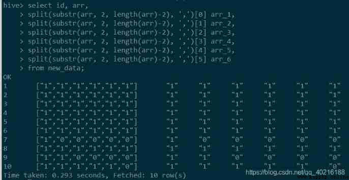
You can see that the final result is in the form of a string , If you want to get a value , You can take another step to intercept 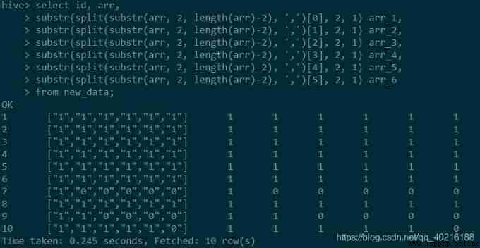
You can see , What we get here is still a string type , and pandas The cast in is similar to ,hive SQL There are also type conversion functions in cast, Use it to force a string to be converted to an integer , The usage method is shown in the following code 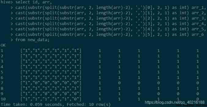
Section :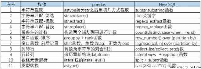
There is an error in the figure : Serial number 7 in : The right is shift function , A positive number is lag, A negative number is lead
import pandas as pd
data = pd.read_excel('order.xlsx')
#data2 = pd.read_excel('order.xlsx', parse_dates=['ts'])
data.head()
data.dtypes
Need to point out that ,pandas Reading data has special support for date types .
Whether in the read_csv In or out read_excel in , There are parse_dates Parameters , You can convert one or more columns in a dataset into pandas Date format in .
data Is read using the default parameters , stay data.dtypes The results of ts The column is datetime64[ns] Format , and data2 Is explicitly specified ts Is a date column , therefore data2 Of ts The type is also datetime[ns].
If the default method is used to read , Date column did not convert successfully , You can use the data2 In such an explicit way .
create table `t_order`(
`id` int,
`ts` string,
`uid` string,
`orderid` string,
`amount` float
)
row format delimited fields terminated by ','
stored as textfile;
load data local inpath 't_order.csv' overwrite into table t_order;
select * from t_order limit 20;
stay hive To load data in, we need to create a table first , Then the data in the text file load Go to the table , The results are shown in the following figure .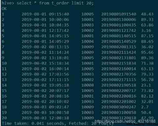
1) Date acquisition
a) Get current date , Mm / DD / yyyy HHM / S
pandas Can be used in now() Function to get the current time , But you need to do another formatting operation to adjust the display format . We add a new list of current time operations to the data set
#pandas
data['current_dt'] = pd.datetime.now()
data['current_dt'] = data['current_dt'].apply(lambda x : x.strftime('%Y-%m-%d %H:%M:%S'))
data.head()
# It's fine too data['current_dt'] = pd.datetime.now().strftime('%Y-%m-%d %H:%M:%S') One step in place
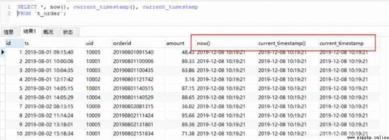
MySQL There are several functions to get the current time :
now(),current_timestamp,current_timestamp(),sysdate(),localtime(),localtime,localtimestamp,localtimestamp() etc. .
#MySQL
SELECT *, now(),current_timestamp(),current_timestamp
FROM `t_order`;
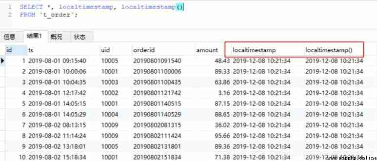
SELECT *, sysdate(),localtime(),localtime
FROM `t_order`;
SELECT *, localtimestamp, localtimestamp()
FROM `t_order`;

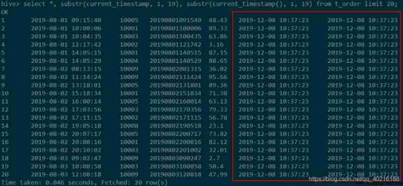
hive Get the current time , have access to current_timestamp(), current_timestamp, What you get is a with milliseconds , If you want to keep the same format as above , Need to use substr Intercept . As shown in the figure below :
#HiveQL
select *, substr(current_timestamp, 1, 19), substr(current_timestamp(), 1, 19)
from t_order limit 20;
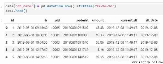
b) Get the current time , Specific date
Follow the ideas of the previous section , Format conversion to get the current date
#pandas
data['dt_date'] = pd.datetime.now().strftime('%Y-%m-%d')
data.head()
#MySQL
SELECT *, curdate() FROM t_order;
#HiveQL
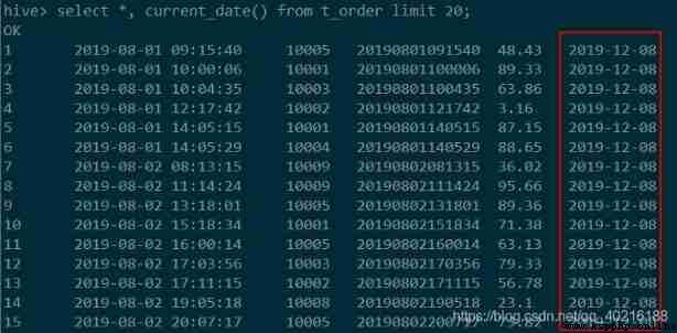
select *, current_date() from t_order limit 20;
c) Extract relevant information from the date
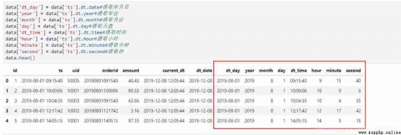
The date includes month, day, hour, minute and second , We can use the corresponding functions to extract . Let's extract ts Days in the field , Time , year , month , Japan , when , branch , Second information .
#pandas
data['dt_day'] = data['ts'].dt.date# Date of withdrawal
data['year'] = data['ts'].dt.year# Year of extraction
data['month'] = data['ts'].dt.month# Extraction month
data['day'] = data['ts'].dt.day# Extraction days
data['dt_time'] = data['ts'].dt.time# Extraction time
data['hour'] = data['ts'].dt.hour# Extraction hours
data['minute'] = data['ts'].dt.minute# Extract minutes
data['second'] = data['ts'].dt.second# Extract seconds
data.head()
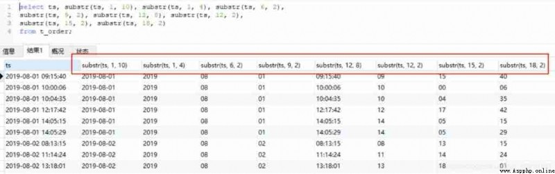
stay MySQL and Hive in , because ts Fields are stored in string format , We just need to use the string interception function . The code for both is the same , Just pay attention to the location and length of the interception
#MySQL
select ts, substr(ts, 1, 10), substr(ts, 1, 4), substr(ts, 6, 2),
substr(ts, 9, 2), substr(ts, 12, 8), substr(ts, 12, 2),
substr(ts, 15, 2), substr(ts, 18, 2)
from t_order;
#HiveQL
select ts, substr(ts, 1, 10), substr(ts, 1, 4), substr(ts, 6, 2),
substr(ts, 9, 2), substr(ts, 12, 8), substr(ts, 12, 2),
substr(ts, 15, 2), substr(ts, 18, 2)
from t_order limit 20;

2) Date conversion
a) The readable date is converted to unix Time stamp
#python
def transfer_time_format(x):
import time
tmp_time = time.strptime(x, '%Y-%m-%d %H:%M:%S')
res_time = int(time.mktime(tmp_time))
return res_time
''' Python time mktime() Function execution and gmtime(), localtime() Reverse operation , It receives struct_time Object as parameter , Returns the floating-point number of seconds for time . mktime() Method syntax :time.mktime(t) Parameters :t -- Structured time or complete 9 Byte element . Return value : Returns the floating-point number of seconds for time . If the value entered is not a legal time , Will trigger OverflowError or ValueError. '''
data['str_ts'] = data['ts'].dt.strftime('%Y-%m-%d %H:%M:%S')
data['str_timestamp'] = data['str_ts'].apply(transfer_time_format)
data.head()
# Writing using anonymous functions
#data['str_timestamp'] = data['str_ts'].apply(lambda x: int(time.mktime(time.strptime(x, '%Y-%m-%d %H:%M:%S'))))
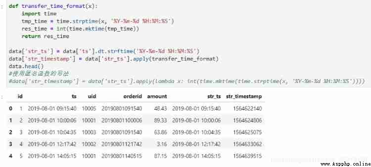
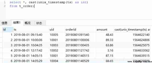
MySQL and Hive You can use the timestamp conversion function in , among MySQL The result is in decimal form , You need to do some type conversion ,Hive Unwanted .
#MySQL
select *, cast(unix_timestamp(ts) as int) from t_order;
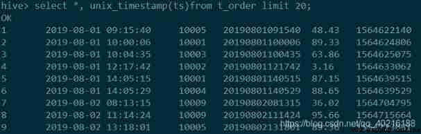
#Hive
select *, unix_timestamp(ts) from t_order limit 20;
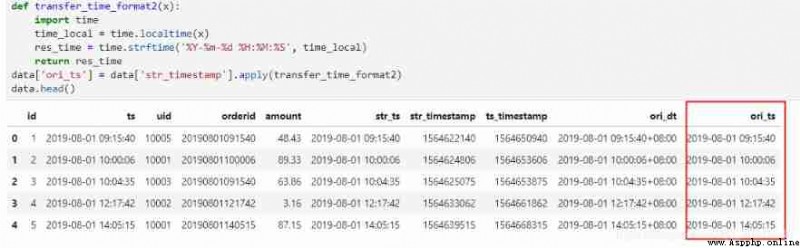
b)unix The timestamp is converted to a readable date
stay pandas in , Let's take a look at how str_timestamp The column is converted to the original ts Column , We still use time Module .
#pandas:
def transfer_time_format2(x):
import time
time_local = time.localtime(x) # take timestamp Convert to local time
res_time = time.strftime('%Y-%m-%d %H:%M:%S', time_local) # Format the time , Convert to time format
return res_time
data['ori_ts'] = data['str_timestamp'].apply(transfer_time_format2)
data.head()
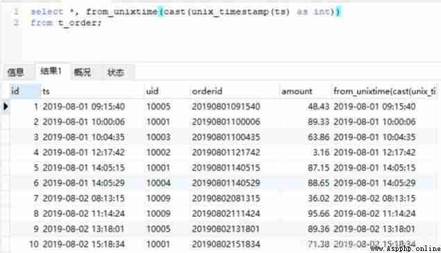
go back to MySQL and Hive, It is still solved with only one function .
#MySQL
select *, from_unixtime(cast(unix_timestamp(ts) as int))
from t_order;
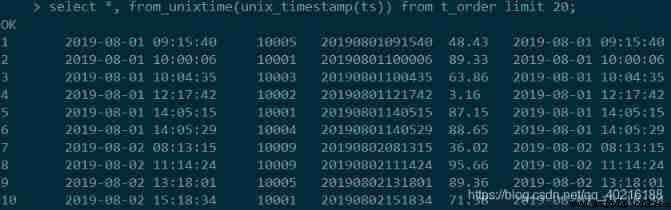
#Hive
select *, from_unixtime(unix_timestamp(ts)) from t_order limit 20;
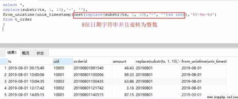
c)10 Bit date to 8 position
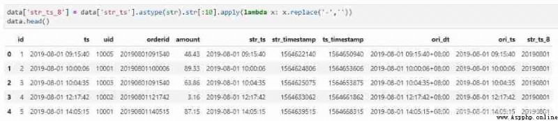
For the initial is ts In the form of month, day, hour, minute and second , We usually need to convert to 10 Format of bit year, month and day , Then replace the horizontal bar in the middle , You can get 8 Bit date .
Due to the intention to replace , Let's first put ts To the form of a string , In the previous conversion , We generated a column str_ts, The data type of the column is object, Equivalent to a string , On this basis, the transformation here can be carried out .
#pandas
data['str_ts_8'] = data['str_ts'].astype(str).str[:10].apply(lambda x: x.replace('-',''))
data.head()
MySQL and Hive It's the same routine in , Interception and replacement are almost the easiest way .
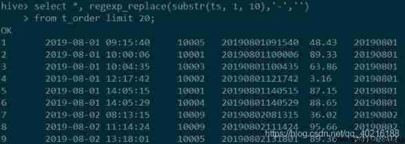
select replace(substr(ts, 1, 10), '-', '') from t_order;
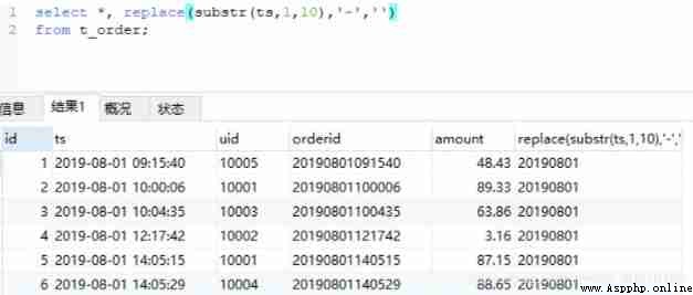
#Hive
select *, regexp_replace(substr(ts, 1, 10),'-','')
from t_order limit 20;
Another way : First convert the string to unix The form of timestamps , Reformat as 8 Date of location .
def transfer_time_format3(x):
import time
time_local = time.localtime(x)
res_time = time.strftime('%Y%m%d', time_local)
return res_time
data['str_ts_8_2'] = data['str_timestamp'].apply(transfer_time_format3)
data.head()

#MySQL
select *, from_unixtime(cast(unix_timestamp(ts) as int), '%Y%M%d')
from t_order;
#Hive
select *, from_unixtime(unix_timestamp(ts),'yyyyMMdd') from t_order limit 20;
d)8 Bit date to 10 position
Method 1 :
#python
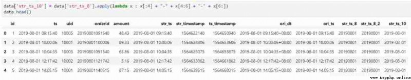
data['str_ts_10'] = data['str_ts_8'].apply(lambda x : x[:4] + "-" + x[4:6] + "-" + x[6:])
data.head()
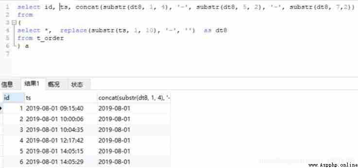
#MySQL
select id, ts, concat(substr(dt8, 1, 4), '-', substr(dt8, 5, 2), '-', substr(dt8, 7,2))
from
(
select *, replace(substr(ts, 1, 10), '-', '') as dt8
from t_order
) a
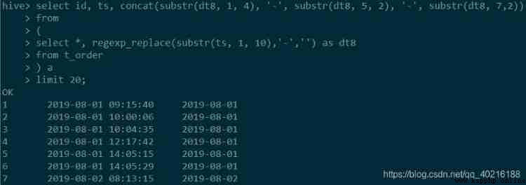
#Hive
select id, ts, concat(substr(dt8, 1, 4), '-', substr(dt8, 5, 2), '-', substr(dt8, 7,2))
from
(
select *, regexp_replace(substr(ts, 1, 10),'-','') as dt8
from t_order
) a
limit 20;
Method 2 :
stay pandas in , With the help of unix Timestamp conversion is inconvenient , We can use datetime Module format function , As shown below .
#pandas
def transfer_time_format4(x):
from datetime import datetime
tmp_time = datetime.strptime('20190801', '%Y%m%d')
res_time = datetime.strftime(tmp_time, '%Y-%m-%d')
return res_time
data['str_ts_10_2'] = data['str_ts_8'].apply(transfer_time_format4)
data.head()

Mysql and Hive in unix_timestamp Different parameters received , The former must be entered as an integer , The latter can be a string . Our goal is to enter a 8 Bit time string , Output one 10 Bit time string . Because there is no 8 Bit time , We constructed a temporary
#MySQL
select *,
replace(substr(ts, 1, 10),'-', ''),
from_unixtime(unix_timestamp(cast(replace(substr(ts, 1, 10),'-', '')as int)),'%Y-%m-%d')
from t_order;
#Hive
select *,
regexp_replace(substr(ts, 1, 10),'-', ''),
from_unixtime(unix_timestamp(regexp_replace(substr(ts, 1, 10),'-', ''), 'yyyyMMdd'),'yyyy-MM-dd')
from t_order
limit 20;

# summary :hive One of the timestamp functions unix_timestamp,from_unixtime
One . date >>>> Time stamp
1.unix_timestamp() Get the current timestamp
for example :select unix_timestamp() --1565858389
2.unix_timestamp(string timestame) The timestamp format entered must be 'yyyy-MM-dd HH:mm:ss', If not, return null
for example :
select unix_timestamp('2019-08-15 16:40:00') --1565858400
select unix_timestamp('2019-08-15') --null
3.unix_timestamp(string date,string pattern) Converts the specified time string format string to unix Time stamp , If not, return null
for example :
select unix_timestamp('2019-08-15','yyyy-MM-dd') --1565798400
select unix_timestamp('2019-08-15 16:40:00','yyyy-MM-dd HH:mm:ss') --1565858400
select unix_timestamp('2019-08-15','yyyy-MM-dd HH:mm:ss') --null
Two . Time stamp >>>> date
1.from_unixtime(bigint unixtime,string format) Convert timestamp to seconds UTC Time , And use a string to represent , It can be done by format Specified time format , Specify the time format of the output , among unixtime yes 10 Bit timestamp value , and 13 The so-called millisecond of bits is not allowed .
for example :
select from_unixtime(1565858389,'yyyy-MM-dd HH:mm:ss') --2019-08-15 16:39:49
select from_unixtime(1565858389,'yyyy-MM-dd') --2019-08-15
2. If unixtime by 13 Bit , It needs to be converted to 10 position
select from_unixtime(cast(1553184000488/1000 as int),'yyyy-MM-dd HH:mm:ss') --2019-03-22 00:00:00
select from_unixtime(cast(substr(1553184000488,1,10) as int),'yyyy-MM-dd HH:mm:ss') --2019-03-22 00:00:00
3、 ... and . Get the current time
select from_unixtime(unix_timestamp(),'yyyy-MM-dd HH:mm:ss') -- 2019-08-15 17:18:55
3) Date calculation
Date calculation mainly includes date interval ( Add or subtract one number to make another date ) And calculate the difference between two dates .
a) Date interval
pandas For the calculation of date interval in, you need to use datetime modular . Let's see how to calculate ts after 5 Days and before 3 God .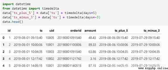
Use timedelta Function can realize the date interval in days , Or by week , minute , Seconds, etc .
stay MySQL and Hive There is a corresponding date interval function in date_add,date_sub function , But the format used is slightly different .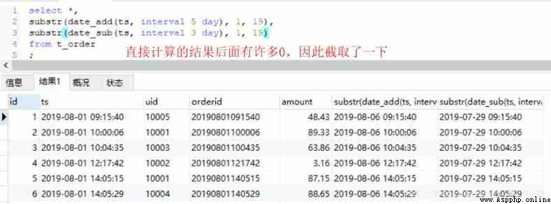
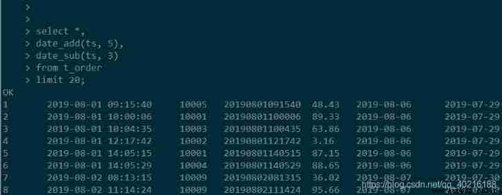
It should be noted that Hive The result of calculation has no time, minute and second , if necessary , It can still be obtained by splicing .
b) Date difference
stay pandas in , If the event type is datetime64[ns] type , The date difference can be obtained by making the difference directly , But there is another one behind the data "days" The unit of , This is actually what was mentioned in the previous section timedelta type .
For ease of use , We use map Function to get its days attribute , Get the difference between the values we want 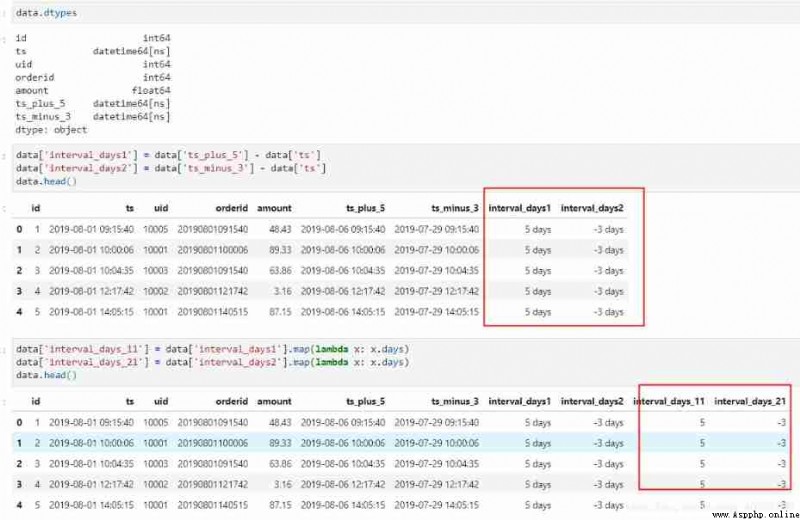
If not datetime Format , You can use the following code to perform a conversion first .
#str_ts It's a string format , Converted dt_ts yes datetime64[ns] Format
data['dt_ts'] = pd.to_datetime(data['str_ts'], format='%Y-%m-%d %H:%M:%S')
Hive and MySQL The date difference in has a corresponding function datediff. But you need to pay attention to its input format .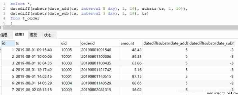
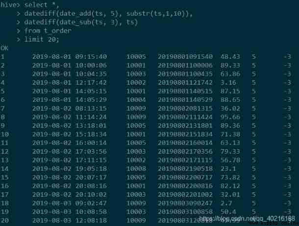
You can see that the input format can be specific to the time, minutes and seconds , It can also be in the format of year, month and day . But be careful Hive The date entered in must be 10 Bit format , Otherwise, the correct result will not be obtained , Such as input 8 Bit , The results will be NULL, and MySQL You can 8 Bit date calculation .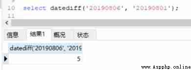
summary :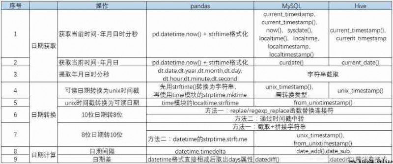
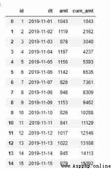
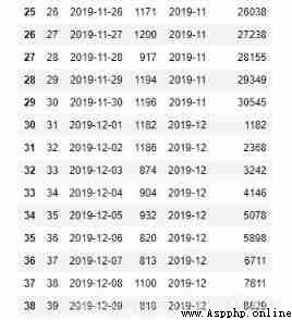
The sample data is as follows , From left to right, it means ,id, date , Current day sales , The data cycle starts from 2019-11-01 To 2019-12-31.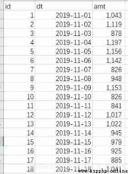
import pandas as pd
import datetime
orderamt = pd.read_excel('orderamt.xlsx')
orderamt.head()
CREATE TABLE `t_orderamt`(
`id` int,
`dt` string,
`orderamt` float)
row format delimited fields terminated by ','
stored as textfile;
load data local inpath 'orderamt.txt' overwrite into table t_orderamt;
select * from t_orderamt limit 20;
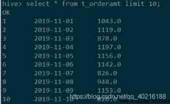
Create the table according to the above code , And then put orderamt.txt Load the contents of into the table , The final data is shown in the figure above .
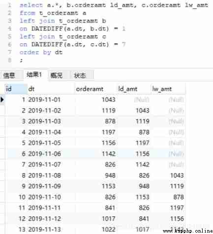
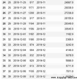
Method 1 : Self correlation , The association condition is that the date difference is 1 and 7, Calculate the current day respectively , yesterday ,7 Data from the day before , Show in three columns , Then you can make a difference and divide to get the percentage .
select a.*, b.orderamt as ld_amt, c.orderamt as lw_amt #as Rename the field , Sometimes you can omit as
from t_orderamt a #t_orderamt The table is named a
left join t_orderamt b
on datediff(a.dt, b.dt)=1 # Find the time interval as 1 God ,a.dt from 2019-11-01 Start , be b.dt from 2019-11-02 Start
left join t_orderamt c
on datediff(a.dt, c.dt)=7
order by dt;
# Associate twice , The conditions are the date difference 1 There is a difference between the day and the date 7 God . If it is not related, leave it blank .
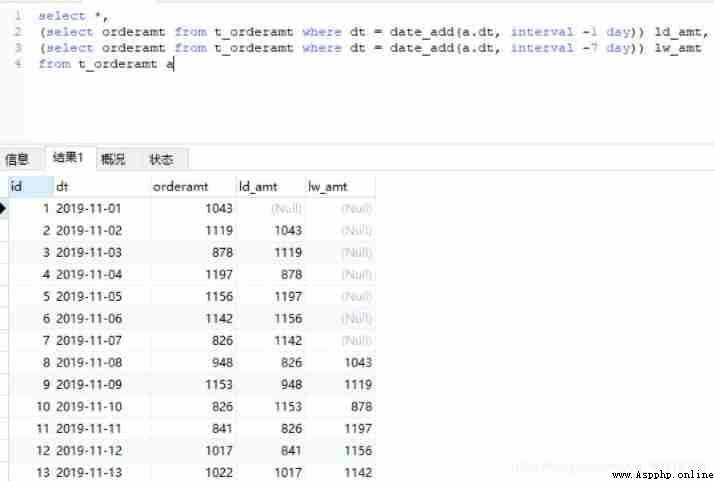
Method 2 : No association , Directly query the data of the previous day and the previous seven days of the current date , The same to 3 Display in the form of columns .
#MySQL
select *,
(select orderamt from t_order where dt=date_add(a.dt, interval 1 day)) ld_amt,
(select orderamt from t_order where dt=date_add(a.dt, interval 7 day)) lw_amt
from t_order a;
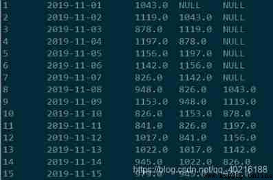
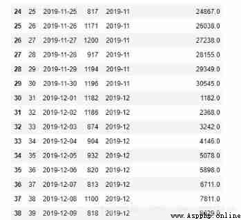
Method 3 : Using window function ,lag
select *,
lag(orderamt, 1) over(order by dt)ld_amt,
lag(orderamt, 7) over(order by dt)lw_amt
from t_orderamt;
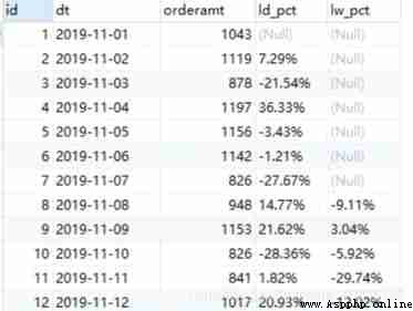
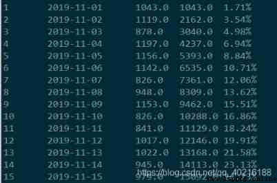
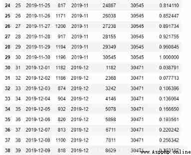
Based on the above code , With a little modification , Increase the code for calculating the percentage , You can get the week-on-week and day on month comparisons respectively .
-- The first paragraph is amended
select a.*, concat(round(((a.orderamt - b.orderamt) / b.orderamt) * 100,2), '%') as ld_pct,
concat(round(((a.orderamt - c.orderamt) / c.orderamt) * 100,2), '%') as lw_pct
from t_orderamt a
left join t_orderamt b
on DATEDIFF(a.dt, b.dt) = 1
left join t_orderamt c
on DATEDIFF(a.dt, c.dt) = 7
order by dt
;
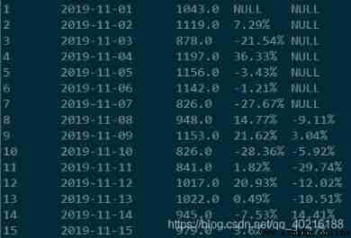
-- The second paragraph is amended
select
b.id, b.dt, b.orderamt,
concat(round(((b.orderamt - ld_amt) / ld_amt) * 100,2), '%') as ld_pct,
concat(round(((b.orderamt - lw_amt) / lw_amt) * 100,2), '%') as lw_pct
from
(
select *,
(select orderamt from t_orderamt where dt = date_add(a.dt, interval -1 day)) ld_amt,
(select orderamt from t_orderamt where dt = date_add(a.dt, interval -7 day)) lw_amt
from t_orderamt a
) b
;
-- The third paragraph is amended
select
b.id, b.dt, b.orderamt,
concat(round(((b.orderamt - ld_amt) / ld_amt) * 100,2), '%') as ld_pct,
concat(round(((b.orderamt - lw_amt) / lw_amt) * 100,2), '%') as lw_pct
from
(
select *, lag(orderamt, 1) over(order by dt) ld_amt,
lag(orderamt, 7) over(order by dt) lw_amt
from t_orderamt
) b
use pandas Calculate
Method 1 : Method of date Association
import pandas as pd
import datetime
orderamt = pd.read_excel('orderamt.xlsx')
#orderamt['dt'] = orderamt['dt'].apply(lambda x: datetime.datetime.strptime(x, '%Y-%m-%d'))# To add and subtract dates , take dt Convert to datetime64[ns] The format of , Run the sentence as appropriate
# Construct two... Respectively dateframe Used to relate
orderamt_plus_1 = orderamt.copy()
orderamt_plus_7 = orderamt.copy()
orderamt_plus_1['dt'] = orderamt_plus_1['dt'] + datetime.timedelta(days=1) # Days plus 1
orderamt_plus_7['dt'] = orderamt_plus_7['dt'] + datetime.timedelta(days=7)
orderamt_1 = pd.merge(orderamt, orderamt_plus_1, on=['dt'],how='left') # A merger
orderamt_1_7 = pd.merge(orderamt_1, orderamt_plus_7, on=['dt'],how='left')
orderamt_all = orderamt_1_7[['id_x', 'dt', 'amt_x', 'amt_y', 'amt']]
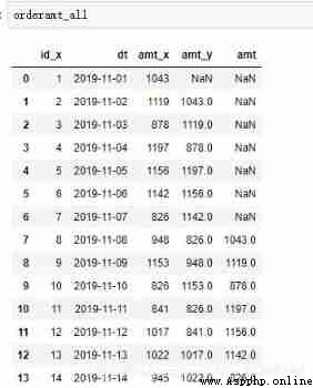
# Connect method 1 code
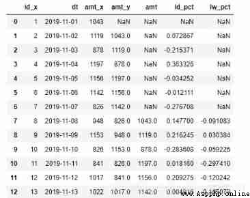
orderamt_all['ld_pct'] = (orderamt_all['amt_x'] - orderamt_all['amt_y']) / orderamt_all['amt_y']
orderamt_all['lw_pct'] = (orderamt_all['amt_x'] - orderamt_all['amt']) / orderamt_all['amt']
orderamt_all
Method 2 : application shift function , Directly select the front n The method
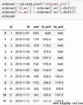
orderamt = pd.read_excel('orderamt.xlsx')
orderamt['ld_amt'] = orderamt['amt'].shift(1)
orderamt['lw_amt'] = orderamt['amt'].shift(7)
orderamt
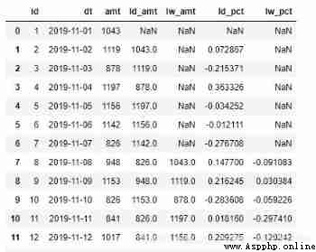
orderamt['ld_pct'] = (orderamt['amt'] - orderamt['ld_amt']) / orderamt['ld_amt']
orderamt['lw_pct'] = (orderamt['amt'] - orderamt['lw_amt']) / orderamt['lw_amt']
orderamt
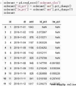
Method 3 : stay pandas in , There are also special functions for calculating the same ring ratio pct_change.
orderamt = pd.read_excel('orderamt.xlsx')
orderamt['ld_pct'] = orderamt['amt'].pct_change()
orderamt['lw_pct'] = orderamt['amt'].pct_change(7)
orderamt
# Formatted string
orderamt['ld_pct'] = orderamt['ld_pct'].apply(lambda x: format(x, '.2%'))
orderamt['lw_pct'] = orderamt['lw_pct'].apply(lambda x: format(x, '.2%'))
orderamt
1) Not grouped
select a.id, a.dt, a.orderamt,
sum(b.orderamt) as cum # Calculate the total amount , use sum function
from t_orderamt a
join t_orderamt b
on a.dt >= b.dt # Non equivalent connection , Because it is cumulative sum , So it has to be >=, if = Words , Seeking is orderamt The sum of
group by a.id, a.dt, a.orderamt;
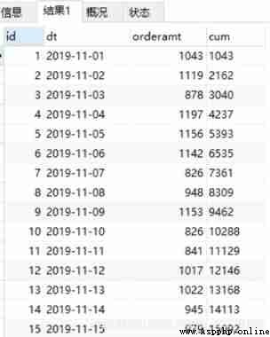
# In the picture cum The column is the cumulative value that we want to request . And the total value of all sales amounts , We can use it directly sum Find out .
select sum(orderamt) as total
from t_orderamt
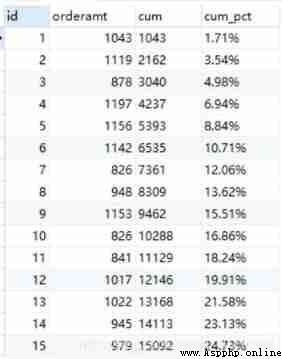
Combine the above two paragraphs SQL, You can get the cumulative percentage , Note that the connection conditions we used 1=1 This constant way . The code and results are as follows
select c.id, c.orderamt, c.cum,
concat(round((c.cum / d.total) * 100, 2), '%') as cum_pct
from
(
select a.id, a.dt, a.orderamt, sum(b.orderamt) as cum
from t_orderamt a
join t_orderamt b
on a.dt >= b.dt
group by a.id, a.dt, a.orderamt
) c
left join
(
select sum(orderamt) as total
from t_orderamt
) d on 1 = 1
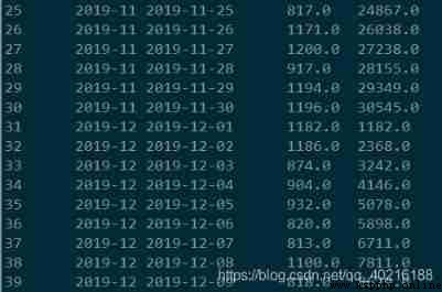
2) Grouping
Now it is necessary to calculate the percentage of daily cumulative sales in the current month
The first is still to calculate the cumulative amount , But it should be accumulated by months . On the basis of the above, add the condition that the months are equal , You can see from the results , stay 11 The month and 12 month cum Columns are accumulated separately .
select substr(a.dt, 1, 7) as mon, a.dt, a.orderamt, sum(b.orderamt) as cum
from t_orderamt a
join t_orderamt b
on a.dt >= b.dt and
substr(a.dt, 1, 7) = substr(b.dt, 1, 7) # Added this condition
group by substr(a.dt, 1, 7), a.dt, a.orderamt
The code for calculating the total amount of each month is relatively simple :
select substr(a.dt, 1, 7) as mon, sum(orderamt) as total
from t_orderamt a
group by substr(a.dt, 1, 7)
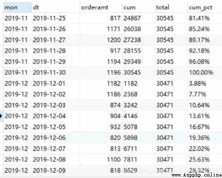
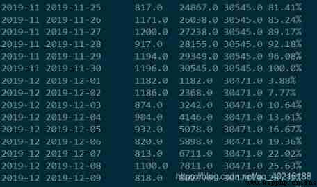
alike , Let's merge the two pieces of code , You will get the cumulative percentage of each month :
select c.mon, c.dt, c.orderamt, c.cum, d.total,
concat(round((c.cum / d.total) * 100, 2), '%') as cum_pct
from
(
select substr(a.dt, 1, 7) as mon, a.dt, a.orderamt, sum(b.orderamt) as cum
from t_orderamt a
join t_orderamt b
on a.dt >= b.dt and substr(a.dt, 1, 7) = substr(b.dt, 1, 7)
group by substr(a.dt, 1, 7), a.dt, a.orderamt
) c
left join
(
select substr(a.dt, 1, 7) as mon, sum(orderamt) as total
from t_orderamt a
group by substr(a.dt, 1, 7)
) d on c.mon = d.mon
1) Not grouped
Hive Does not support the on Join conditions with unequal sign in , Although it can be used where The way to transform , The code is as follows . But this is not the best solution . We can use Hive Window function in , It is very convenient to calculate the cumulative value .
#where Method
select a.id, a.dt, a.orderamt,
sum(b.orderamt) as cum-- Yes b Sum the amounts in the table
from t_orderamt a
join t_orderamt b
on 1=1
where a.dt >= b.dt-- Use unequal connection
group by a.id, a.dt, a.orderamt
# Window function
select *, sum(orderamt) over(order by dt) as cum from t_orderamt;
The results are the same 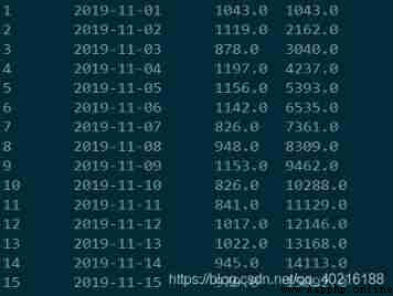
Next, let's focus on how window functions work . When calculating the total value and before MySQL In a similar way , The calculation of cumulative percentage also needs to combine the two parts of code .
select c.id, c.dt, c.orderamt, c.cum,
concat(round((c.cum / d.total) * 100, 2), '%') as cum_pct
from
(
select *, sum(orderamt) over(order by dt) as cum
from t_orderamt
) c
left join
(
select sum(orderamt) as total
from t_orderamt
) d
on 1 = 1-- stay Hive This condition may not be written
2) Grouping
The situation of grouping , In the window function, you can use partition by Directly specify the grouped , See the following code
select id, substr(dt, 1, 7) as mon,
dt, orderamt,
sum(orderamt) over(partition by substr(dt, 1, 7) order by dt) as cum
from t_orderamt;
You can see , The same as the previous grouping , stay 11 The month and 12 month cum Columns are accumulated separately .
Next, it's easy to write the code to calculate the cumulative percentage by grouping , The result is consistent with the above .
select c.mon, c.dt, c.orderamt, c.cum, d.total,
concat(round((c.cum / d.total) * 100, 2), '%') as cum_pct
from
(
select id, substr(dt, 1, 7) as mon, dt, orderamt, sum(orderamt) over(partition by substr(dt, 1, 7) order by dt) as cum
from t_orderamt
) c
left join
(
select substr(dt, 1, 7) as mon, sum(orderamt) as total
from t_orderamt
group by substr(dt, 1, 7)
) d on c.mon = d.mon
stay pandas in , A special function is provided to calculate the cumulative value , Namely cumsum function ,expanding function ,rolling function . Let's take a look at how to calculate the cumulative percentage of grouped and ungrouped using three functions .
1) Not grouped
a)cumsum function
cumsum yes pandas A function used to calculate the cumulative sum . Similar functions include cumprod Calculate cumulative product ,cummax Before calculation n The maximum value of a value ,cummin Before calculation n The minimum of values .
import pandas as pd
orderamt = pd.read_excel('orderamt.xlsx')
orderamt['cum_amt'] = orderamt['amt'].cumsum()
orderamt.head(15)
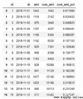
orderamt['cum_amt_pct'] = orderamt['cum_amt'] / orderamt['amt'].sum()
orderamt.head(15)
b)expanding function
pandas Medium expanding Function is a kind of window function , It does not fix the size of the window , It's a cumulative calculation . Be similar to cumsum(), But more powerful .
orderamt = pd.read_excel('orderamt.xlsx')
orderamt['mon'] = orderamt['dt'].dt.strftime('%Y-%m')# Get the month in string form
orderamt['cum_expand'] = orderamt.expanding(min_periods=1)['amt'].sum()
orderamt.head(15)
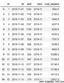
Parameters min_periods Represents the smallest observation window , The default is 1, Can be set to other values , But if the number of records in the window is less than this value , Is displayed NA.
With the cumulative value , Calculate the cumulative percentage , May, in accordance with the cumsum The method in , Omit here .
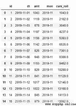
c)rolling function
rolling Function and expanding comparison , It mainly fixes the window size . When the window exceeds dataframe When the length of the , Can be realized with expanding The same effect . The above code is used rolling Function can be rewritten as follows , Note that window Parameter is len(orderamt):
orderamt = pd.read_excel('orderamt.xlsx')
orderamt['mon'] = orderamt['dt'].dt.strftime('%Y-%m')# Get the month in string form
orderamt['cum_roll'] = orderamt.rolling(window=len(orderamt), min_periods=1)['amt'].sum()
orderamt.head(15)
2) Grouping
a)cumsum function
# add to pandas Display settings , Show all lines
pd.set_option('display.max_rows', None)
orderamt = pd.read_excel('orderamt.xlsx')
orderamt['mon'] = orderamt['dt'].dt.strftime('%Y-%m')
# After grouping amt Find the cumulative sum
orderamt['cum_mon'] = orderamt.groupby('mon')['amt'].cumsum()
orderamt
Next, calculate the total value of the group , It's used here pandas Medium transform function , The total value calculated after grouping can be written into the original dataframe.
orderamt['mon_total'] = orderamt.groupby('mon')["amt"].transform('sum')
orderamt['grp_cum_pct'] = orderamt['cum_mon'] / orderamt['mon_total']
orderamt
b)expanding function
Use... In group situations expanding Function needs and groupby combination , Notice that the result is multiple indexes , Need to take values Can be assigned to the original dataframe.
orderamt = pd.read_excel('orderamt.xlsx')
orderamt['mon'] = orderamt['dt'].dt.strftime('%Y-%m')
orderamt_mon_group = orderamt.groupby('mon').expanding(min_periods=1)['amt'].sum()
# there orderamt_mon_group The index has two sides , Let's take values The value of can be the same as the original dataframe Splice together
orderamt['orderamt_mon_group'] = orderamt_mon_group.values
orderamt
c)rolling function
rolling Function and expanding The code of the function is almost the same , Need to add window Parameters .
orderamt = pd.read_excel('orderamt.xlsx')
orderamt['mon'] = orderamt['dt'].dt.strftime('%Y-%m')
orderamt_mon_group_roll = orderamt.groupby('mon').rolling(len(orderamt),min_periods=1)['amt'].sum()
# there orderamt_mon_group_roll The index has two sides , Let's take values The value of can be the same as the original dataframe Splice together
orderamt['orderamt_mon_group_roll'] = orderamt_mon_group_roll.values
orderamt
The data in this paper are dated :
https://www.kaggle.com/nikhil04/login-time-for-users .
The data format is relatively simple :id: Self increasing id,uid: The only user id.ts: User login time ( Accurate to seconds ), The data sample is shown in the figure below .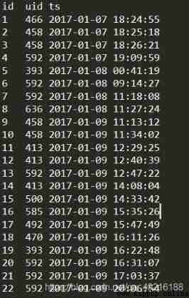
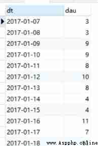
Here, we agree that daily work refers to logging in every day user_id Go and count , From our data , The calculation is very simple .
As early as in the first part of the series, we learned group by Aggregation operation . Just group by day , take uid To count again , You get the answer . The code is as follows :
select substr(ts, 1, 10) as dt, count(distinct uid) as dau
from t_login
group by substr(ts, 1, 10);
import pandas as pd
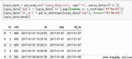
login_data = pd.read_csv('login_data.txt', sep='\t', parse_dates=['ts'])
login_data.head()
login_data['day'] = login_data['ts'].map(lambda x: x.strftime('%Y-%m-%d'))
uid_count = login_data.groupby('day').aggregate({
'uid': lambda x: x.nunique()})
uid_count.reset_index(inplace=True)
uid_count

Retain It's a dynamic concept , It refers to the users who have used the product for a certain period of time , Users who are still using the product after a period of time , The retention rate can be calculated by comparing the two . The common retention rate is the next day retention rate ,7 Daily retention rate ,30 Daily retention rate, etc . Next day retention refers to the active users today , How many active users are left tomorrow . The higher the retention rate , It means that the stickiness of the product is better .
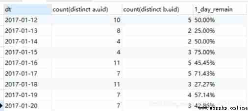
Retention rate refers to the proportion of users who still log in after a period of time in the first day of login , because 2017-01-07 Too few users are logged in , We choose 2017-01-12 As the first day . Calculate the retention rate of the next day respectively ,7 Japan ,14 Daily retention rate .
select substr(a.ts, 1, 10) as dt,
count(distinct a.uid), count(distinct b.uid),
concat(round((count(distinct a.uid) / count(distinct b.uid))*100, 2), %)
from t_login a
left join t_login b
on a.uid=b.uid
and date_add(substr(a.ts, 1, 10), interval 1 day)=substr(b.ts, 1, 10)
group by substr(a.ts, 1, 10);
b) Multi day retention calculation
When the amount of data is large ,join It will be inefficient
select sunstr(a.dt, 1, 10) as dt,
count(distinct a.uid),
count(distinct if(datediff(substr(b.ts, 1, 10), substr(a.ts, 1, 10))=1, b.uid, null)) as 1_day_remain_uid,
count(distinct if(datediff(substr(b.ts, 1, 10), substr(a.ts, 1, 10))=6, b.uid, null)) as 7_day_remain_uid,
count(distinct if(datediff(substr(b.ts, 1, 10), substr(a.ts, 1, 10))=13, b.uid, null)) as 14_day_remain_uid
from t_login a
left join t_login b
on a.uid=b.uid
group by substr(a.ts, 1, 10)
As the code shows , When associating, do not limit the date first , When querying the outermost layer, you can limit the date difference according to your own goal , The corresponding number of retained users can be calculated , Active users on the first day can also be regarded as the date difference is 0 The case when . In this way, you can calculate the retention for multiple days at one time . give the result as follows , If you want to calculate the retention rate , Just convert to the corresponding percentage , Refer to the previous code , Here slightly .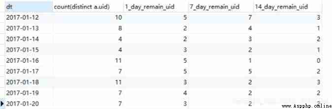
Import data and add two columns of dates , They are string format and datetime64 Format , It is convenient for subsequent date calculation
import pandas as pd
from datetime import datetime
login_data=pd.read_csv('login_data.txt', sep='\t', parse_dates=['ts'])
login_data['day']=login_data['ts'].map(lambda x: x.strftime('%Y-%m-%d'))
login_data['dt_ts']=pd.to_datetime(login_data['day'], format='%Y-%m-%d'))
login_data.head()
Construct new dataframe, Calculate the date , Then connect with the original data .
data_1=login_data.copy()
data_1['dt_ts_1']data['dt_ts']+timedelta(-1)
data_1.head()

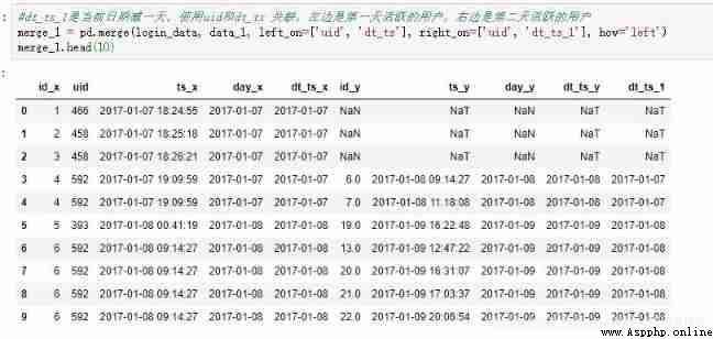
Merge the previous two data , Use uid and dt_ts relation ,dt_ts_1 Is the current date minus one day , On the left are active users on the first day , On the right are the active users the next day
merge_1=pd.merge(login_data, data_1, left_on=['uid', 'dt_ts'], right_on=['uid', 'dt_ts_1'], how='left')
merge_1.head()
Calculate the number of active users on the first day
init_user = merge_1.groupby('day_x').aggregate({
'uid': lambda x: x.nunique()})
init_user.reset_index(inplace=True)
init_user.head()
Calculate the number of active users in the next day
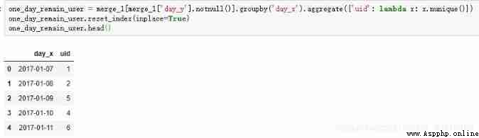
one_day_remain_user = merge_1[merge_1['day_y'].notnull()].groupby('day_x').aggregate({
'uid': lambda x: x.nunique()})
one_day_remain_user.reset_index(inplace=True)
one_day_remain_user.head()
Combine the results of the previous two steps , Calculate the final retention
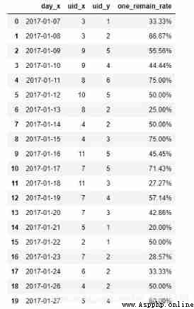
merge_one_day = pd.merge(init_user, one_day_remain_user, on=['day_x'])
merge_one_day['one_remain_rate'] = merge_one_day['uid_y'] / merge_one_day['uid_x']
merge_one_day['one_remain_rate'] = merge_one_day['one_remain_rate'].apply(lambda x: format(x, '.2%'))
merge_one_day.head(20)
b) Multi day retention calculation
Method 1 :
Calculate the date difference , Prepare for the follow-up
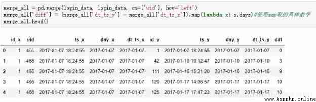
merge_all = pd.merge(login_data, login_data, on=['uid'], how='left')
merge_all['diff'] = (merge_all['dt_ts_y'] - merge_all['dt_ts_x']).map(lambda x: x.days)# Use map Get specific figures
merge_all.head()
Computation first n Days of retention ,n=0,1,6,13. You need to filter before counting , Still use nunique
diff_0 = merge_all[merge_all['diff'] == 0].groupby('day_x')['uid'].nunique()
diff_1 = merge_all[merge_all['diff'] == 1].groupby('day_x')['uid'].nunique()
diff_6 = merge_all[merge_all['diff'] == 6].groupby('day_x')['uid'].nunique()
diff_13 = merge_all[merge_all['diff'] == 13].groupby('day_x')['uid'].nunique()
diff_0 = diff_0.reset_index()#groupby After counting, we get series Format ,reset obtain dataframe
diff_1 = diff_1.reset_index()
diff_6 = diff_6.reset_index()
diff_13 = diff_13.reset_index()
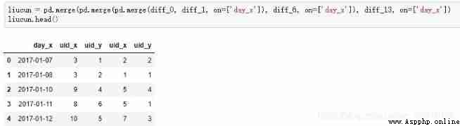
For many dataframe Make a merger
liucun = pd.merge(pd.merge(pd.merge(diff_0, diff_1, on=['day_x'], how='left'), diff_6, on=['day_x'], how='left'), diff_13, on=['day_x'], how='left')
liucun.head()
Rename the result , And use 0 fill na value
liucun.columns=['day', 'init', 'one_day_remain', 'seven_day_remain', 'fifteen_day_remain']
liucun.fillna(0, inplace=True)
liucun.head(20)
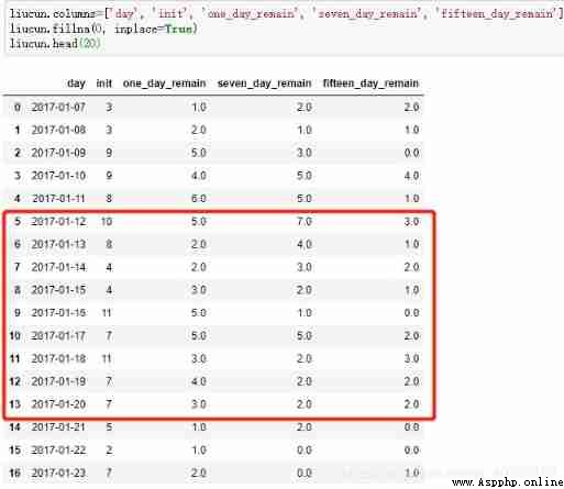
The results and SQL The calculation is consistent , The code for percentage conversion is also omitted .
Method 2 :
def cal_n_day_remain(df, n):
dates = pd.Series(login_data.dt_ts.unique()).sort_values()[:-n]# Take until n The date of day , Guaranteed n Daily retention
users = [] # Define the initial number of users stored in the list
remains = []# Define the number of reserved users stored in the list
for d in dates:
user = login_data[login_data['dt_ts'] == d]['uid'].unique()# Active users of the day
user_n_day = login_data[login_data['dt_ts']==d+timedelta(n)]['uid'].unique()#n Active users in the future
remain = [x for x in user_n_day if x in user]# intersect
users.append(len(user))
remains.append(len(remain))
# A cycle of one day n Daily retention
# Construct after the loop ends dataframe And back to
remain_df = pd.DataFrame({
'days': dates, 'user': users, 'remain': remains})
return remain_df
one_day_remain = cal_n_day_remain(login_data, 1)
seven_day_remain = cal_n_day_remain(login_data, 6)
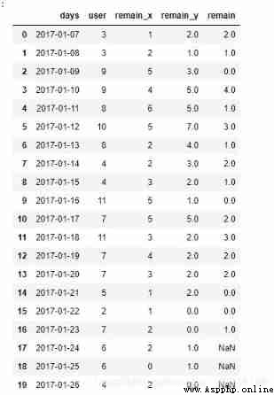
fifteen_day_remain = cal_n_day_remain(login_data, 13)
liucun2 = pd.merge(pd.merge(one_day_remain, seven_day_remain[['days', 'remain']], on=['days'], how='left'), fifteen_day_remain[['days', 'remain']], on=['days'], how='left')
liucun2.head(20)
brief introduction :
pandasql By Yhat Written simulation R package sqldf Of python Third party Library , Can let us use SQL How to operate pandas Data structure of .
install :
Use on the command line pip install pandasql Can be installed .
Use :
from pandasql Packages can be imported sqldf, This is the interface to be used by our core . It takes two parameters , The first is legal SQL sentence .SQL Functions , For example, aggregation , Conditions of the query , coupling ,where Conditions , Sub query and so on , It all supports . The second is locals() perhaps globals() Represents the environment variable , It will identify the existing dataframe As the table name in the first parameter .
import pandas as pd
from pandasql import sqldf#d Import sqldf
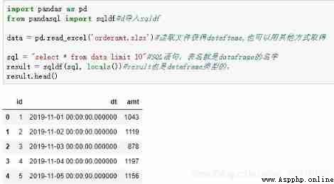
data = pd.read_excel('orderamt.xlsx')# Read the file to get dataftame, It can also be obtained in other ways
sql = "select * from data limit 10"#SQL sentence , The name of the watch is dataframe Name
result = sqldf(sql, locals())#result It's also dataframe Type of ,
result.head()
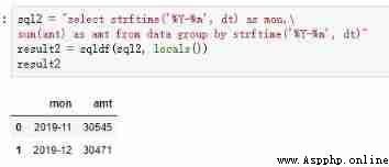
Monthly aggregation :
sql2 = "select strftime('%Y-%m', dt) as mon,\
sum(amt) as amt from data group by strftime('%Y-%m', dt)"
result2 = sqldf(sql2, locals())
result2
The official document says that in order to avoid redundant calls, the sqldf Make a layer of encapsulation , use pysqldf Instead of , Just pass in a SQL Statement parameters , As shown in the following code . But I tried not to package it . The previous code can be omitted locals() perhaps globals().
pysqldf = lambda q: sqldf(q, globals())
result = pysqldf(sql)# Pass in legal SQL sentence
Use custom SQL obtain dataframe after , Can continue to use pandas Handle , You can also save it directly .
1)pandas operation MySQL database
read_sql:
The function is , Run against tables in the database SQL sentence , Change the query results to dataframe The format returns . There are two more read_sql_table,read_sql_query, Usually use read_sql That's enough . The two main parameters are legal SQL Statement and database connection . Data links can use SQLAlchemy Or string . For other optional parameters, please refer to the official documentation .
to_sql:
The function is , take dataframe Results of are written to the database . Provide the table name and connection name , There is no need to create a new MySQL surface .
Use operation MySQL Examples are as follows , Need to be installed in advance sqlalchemy,pymysql, direct pip Can be installed , We need to pay attention to engine The format of .
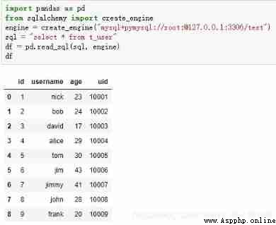
#read_sql give an example
import pandas as pd
from sqlalchemy import create_engine
engine = create_engine("mysql+pymysql://root:[email protected]:3306/test")
# The user name of the database :root, password :123456,host:127.0.0.1, port :3306, Database name :test
#engine = create_engine("dialect+driver://username:[email protected]:port/database")
sql = "select * from t_user"
df = pd.read_sql(sql, engine)
df
#to_sql give an example
df2 = df.head()
df2.to_sql('t_user_2', engine, index=None)
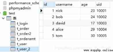
t_user_2 Is the result table name , There is no need to build in the database in advance , Otherwise, an error will be reported , The field name of the table is dataframe Column name of .engine Is the connection created above .df2 Is the data expected to be written , Only the above is selected here df The first five elements of . It should be noted that if you do not add index=None Parameters , Will put the index in , One more column index.