polynomial Logical regression It is an extension of logistic regression , It adds support for multi class classification problems .
By default , Logistic regression is limited to two types of classification problems . Some extensions , Logistic regression can be used for multi class classification problems , Although they require that the classification problem be transformed into multiple binary classification problems first .
contrary , Multinomial logistic regression algorithm is an extension of logistic regression model , It involves changing the loss function to cross entropy loss , The probability distribution is predicted as a multiple probability distribution , Support multi class classification problems with native .
In this tutorial , You will learn how to Python Develop multiple logistic regression models in .
After completing this tutorial , You will learn :
This tutorial is divided into three parts :
Logical regression is a classification algorithm .
It is applicable to data sets with digital input variables and classification target variables with two values or classes . This type of problem is called binary classification problem .
Logistic regression is designed for two kinds of problems , Use binomial probability distribution function . For positive classes or results , Class labels map to 1, For negative classes or results , Mapping to 0. The prediction example of the fitting model belongs to the 1 The probability of a class .
By default , Logistic regression cannot be used for classification tasks with more than two category labels , The so-called multi category classification .
contrary , It needs to be modified to support multi class classification problems .
A popular way to adapt logistic regression to multi class classification problems is to divide multi class classification problems into multiple binary classification problems , The standard logistic regression model is fitted on each sub problem .
Another approach involves changing the logistic regression model to directly support the prediction of multiple category labels . say concretely , Predict the probability that the input example belongs to each known class label .
The probability distribution that defines multiple kinds of probability is called multiple probability distribution . The logistic regression model suitable for learning and predicting multiple probability distributions is called multiple logistic regression . Again , We can call default or standard logistic regression binomial logistic regression .
Change the logistic regression from binomial probability to polynomial probability , You need to change the loss function used to train the model ( for example , Change logarithmic loss to cross entropy loss ), The output is changed from a single probability value to a probability of each class label .
Now we are familiar with multiple logistic regression , Let's see how we can Python Develop and evaluate multiple logistic regression models .
In this section , We will use Python The machine learning library develops and evaluates a multiple logistic regression model .
First , We will define a synthetic multi class classification dataset , As the foundation . This is a general data set , In the future, you can easily replace... With the data set you load yourself .
classification() Function can be used to generate a number of rows 、 Data sets of columns and classes . under these circumstances , We will generate a with 1000 That's ok 、10 Input variables or columns and 3 A data set of classes .
The following example summarizes the shape of the array and the example distribution in the three classes .
#  Test classification dataset
import Counter
#  Define datasets
X, y = mclas
#  Summarize the data set
print
Run this example , It is confirmed that the data set has 1,000 Row sum 10 Column , As we expected , And these rows are roughly evenly distributed among the three categories , There are about... In each category 334 An example .

scikit Library support Logistic Return to .
take "solver " The parameter is set to the solver that supports multi index logistic regression , So it can be configured as multi index logistic regression .
#  Define polynomial logistic regression model
modl = LoRe(muss)
Polynomial logistic regression models will be fitted using cross entropy loss , The integer value of each integer encoded class label will be predicted .
Now we are familiar with multiple logistic regression API, We can see how to evaluate a multiple logistic regression model on our synthetic multiclass classification dataset .
Use repeatedly layered k-fold Cross validation is a good practice to evaluate classification models . Layering ensures that the distribution of examples in each category of each cross validation fold is roughly the same as that of the whole training data set .
We will use 10 Three fold repetitions , This is a good default , And considering the balance of classes , Use classification accuracy to evaluate model performance .
A complete example of multiple logistic regression for evaluating multiclass classification is listed below .
#  Evaluate multiple indicators Logistic The regression model
from numpy import mean
#  Define datasets
X, y = makeclas
#  Define polynomial logistic regression model
modl = LogReg
#  Define the evaluation procedure of the model
cv = RepeKFold
#  Evaluate the model and collect scores
n_scores = crovalsc
#  Report the performance of the model
print('Mean Accurac)
Running this example can report the average classification accuracy of all cross validation and evaluation procedures .
Be careful : Given the randomness of the algorithm or evaluation program , Or the difference in digital accuracy , Your results may be different . Consider running this example several times , Then compare the average results .
In this case , We can see , On our synthetic classification dataset , The multinomial logistic regression model with default penalty achieves about 68.1% Average classification accuracy .

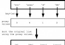
We can decide to use multiple logistic regression model as our final model , And predict the new data .
This can be done by first fitting the model on all available data , And then call predict() Function to predict new data .
The following example demonstrates how to use multiple logistic regression models to predict new data .
#  Multi index logistic regression model was used for prediction
from sklearn.datasets
#  Define datasets
X, y = makclas
#  Define polynomial logistic regression model
model = LogRegr
#  Fit the model on the whole data set
fit(X, y)
#  Define single line input data
row
#  Forecast category label
predict(\[row\])
#  Summarize the predicted classes
print('Predic
To run this example, first fit the model on all available data , Then define a row of data , Provide to the model , In order to predict .
under these circumstances , We can see , The prediction of the model for single line data is "1 " class .

One advantage of polynomial logistic regression is , It can predict the calibration probability of all known class labels in the data set .
This can be done by calling the... Of the model predict_proba() Function to implement .
The following example demonstrates how to use the multiple logistic regression model to predict the multiple probability distribution of a new example .
#  The probability is predicted by multi index logistic regression model
from sklea
#  Define datasets
X, y = makclassif
#  Define polynomial logistic regression model
model = LoRegre
#  Fit the model on the whole data set
fit(X, y)
#  Define single line input data
#  Predict a polynomial probability distribution
preprob
#  Summarize the predicted probability
print('Predict
To run this example, first fit the model on all available data , Then define a row of data , Provide it to the model , In order to predict the probability of the class .
Be careful : Given the randomness of the algorithm or evaluation program , Or the difference in digital accuracy , Your results may be different . Consider running this example several times , And compare the average results .
In this case , We can see the 1 class ( for example , The array index is mapped to the integer value of the class ) The probability of prediction is the highest , about 0.50.

Now we are familiar with evaluating and using multiple logistic regression models , Let's explore how to adjust the hyperparameters of the model .
An important super parameter for adjusting multiple logistic regression is the penalty term .
This term imposes a penalty on the model , Seek smaller model weights . This is achieved by adding the weighted sum of model coefficients to the loss function , Encourage the model to reduce the weight and error while fitting the model .
A popular type of punishment is L2 punishment , It sums the squares of the coefficients ( weighting ) Add to the loss function . Weighting of coefficients can be used , Reduce the intensity of punishment from complete punishment to very slight punishment .
By default ,LogisticRegression Class uses L2 punishment , The weight of the coefficient is set to 1.0. The type of punishment can be determined by " punishment " Parameter setting , Its value is "l1"、"l2"、"elasticnet"( For example, both ), Although not all solvers support all penalty types . The coefficient weight in the penalty can be calculated by "C " Parameter setting .
#  Define a polynomial logistic regression model with default penalty
Logistic
The weighting of punishment is actually inverse weighting , Maybe punishment =1-C.
As can be seen from the document .
C : float, default=1.0The reciprocal of the regularization strength , Must be a positive floating point number . Like support vector machines , A smaller value indicates a stronger penalty .
It means , near 1.0 The value of indicates little penalty , near 0 The value of represents a strong penalty .C The value is 1.0 It may mean that there is no punishment at all .
#  Define a penalty free polynomial logistic regression model
LogRegr( penal='none')
Now we are familiar with punishment , Let's see how to explore the impact of different penalty values on the performance of multi index logistic regression model .
It is common to test penalty values on a logarithmic scale , In this way, we can quickly find a very effective penalty scale for a model . Once found , Further adjustment on this scale may be beneficial .
We will explore weighted values on a logarithmic scale 0.0001 To 1.0 Between L2 punishment , There is also impunity or 0.0.
The following lists the methods used to evaluate multiple logistic regression L2 A complete example of penalty values .
# Adjust the regularization of multi index logistic regression
from numpy import mean
# Get data set
def getet():
X, y = make_
# Get a list of models to evaluate
def ges():
models = dict()
# Create a name for the model
# In some cases, turn off punishment
# In this case, there is no punishment
models\[key\] = LogisticReg penalty='none'
models\[key\] = LogisticR penalty='l2'
# Use cross validation to evaluate a given model
def evamodel
# Define the evaluation procedure
cv = RataifiFod
# Evaluation model
scs= cssva_scre
# Define datasets
X, y = gatet()
# Get the model to evaluate
gt_dels()
# Evaluate the model and store the results
for name, moel in mos.ims():
# Evaluate the model and collect scores
oes = evadel(model, X, y)
# Store results
rsts.append
names.append
# summary
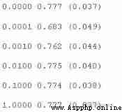
# Draw a comparison chart of model performance Run this example to report the average classification accuracy of each configuration .
Be careful : Given the randomness of the algorithm or evaluation program , Or the difference in digital accuracy , Your results may be different . Consider running this example a few more times , And compare the average results .
In this case , We can see ,C The value is 1.0 The best score is about 77.7%, This is the same as achieving the same score without penalty .
A box whisker diagram is created for the accuracy score of each configuration , All graphs are displayed side by side on a graph of the same scale , For direct comparison .
under these circumstances , We can see , The greater the penalty we use on this dataset ( namely C The smaller the value. ), The worse the performance of the model .
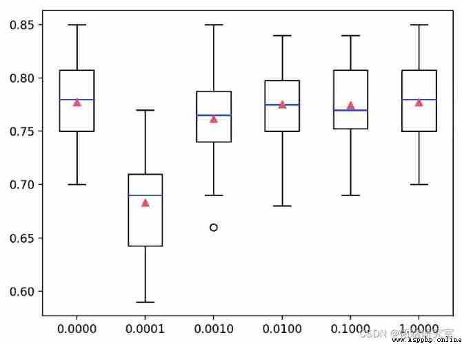
polynomial Logistic Returning L2 Box diagram of punishment and accuracy
In this tutorial , You've learned how to Python Develop multiple logistic regression models in .
Do you have any questions ?
Ask your questions in the comments below , I will try my best to answer .

The most popular insights
1.R Language diversity Logistic Logical regression The application case
2. Panel smooth transfer regression (PSTR) Analyze the case and realize Analyze the case and realize ")
3.matlab Partial least squares regression in (PLSR) And principal component regression (PCR)
4.R Language Poisson Poisson Regression model analysis case
5.R Language mixing effect logistic regression Logistic Model analysis of lung cancer
6.r In language LASSO Return to ,Ridge Ridge return and Elastic Net Model implementation
7.R Logical regression of language 、Naive Bayes Bayes 、 Decision tree 、 Random forest algorithm predicts heart disease
8.python Using linear regression to predict stock prices
9.R Language uses logical regression 、 Decision tree and random forest are used to classify and predict credit data sets