python Analysis of the catering industry for actual project analysis
For orders order_id
Analyze for time and date
technology ( Data analysis in different dimensions )
For orders order_id:
Analyze for time and date :
Technical point :
For orders order_id
# Load data
import pandas as pd
import numpy as np
import matplotlib.pyplot as plt
plt.rcParams['font.sans-serif']=['SimHei'] # Show Chinese tags
#plt.rcParams['axes.unicode_minus']=False # These two lines need to be set manually
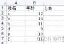
data1=pd.read_excel('D:\\zhangxinfile\\python Data practice (jupyter lab)\\ Data analysis and actual project data \ The restaurant \\meal_order_detail.xlsx',sheet_name='meal_order_detail1')
data2=pd.read_excel('D:\\zhangxinfile\\python Data practice (jupyter lab)\\ Data analysis and actual project data \ The restaurant \\meal_order_detail.xlsx',sheet_name='meal_order_detail2')
data3=pd.read_excel('D:\\zhangxinfile\\python Data practice (jupyter lab)\\ Data analysis and actual project data \ The restaurant \\meal_order_detail.xlsx',sheet_name='meal_order_detail3')
data=pd.concat([data1,data2,data3],axis=0)
#data.info()
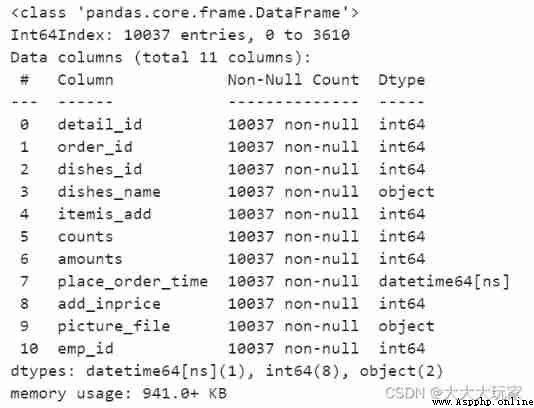
#2. Data preprocessing ( Merge data ,NA Handle ), Analyze the data
data.dropna(axis=1,inplace=True)
data.info()
# Count the average price of dishes sold
round(data['amounts'].mean(),2)
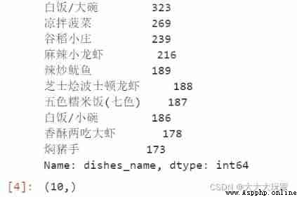
# frequency statistic , What dish is the most popular ( Make statistics on the frequency of dish names , Take the top ten )
dishes_count=data['dishes_name'].value_counts()[0:10]
print(dishes_count)
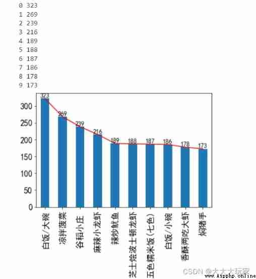
# Data visualization
dishes_count.shape# View as one-dimensional data
dishes_count.plot(kind='line',color='red')
dishes_count.plot(kind='bar',fontsize='16')# The receipt bar chart can
for x,y in enumerate(dishes_count): # Add words
print(x,y)
plt.text(x,y+2,y,ha='center',fontsize='12')
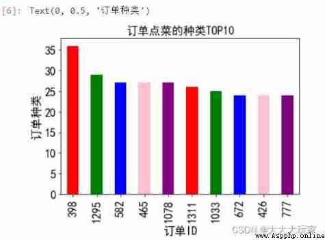
# Orders have the most types of dishes ( The kind and quantity are different )
data_group = data['order_id'].value_counts()[0:10]
data_group.plot(kind='bar',fontsize='16',color=['red','green','blue','pink','purple'])
plt.title(' Type of order TOP10',fontsize='16')
plt.xlabel(' Order ID',fontsize='16')
plt.ylabel(' Order type ',fontsize='16')
#8 Before the order of restaurant in January 10 name , Average order 25 A dish
# Order ID Order the most ( grouping order_id,counts Sum up , Sort , The top ten )
data['total_amounts']=data['counts']*data['amounts']# Count the total consumption of a single dish
dataGroup= data[['order_id','counts','amounts','total_amounts']].groupby(by='order_id')
Group_sum=dataGroup.sum()# Grouping sum , according to order_id Perform group sum and separate sum counts Harmony of amounts And ,total_amounts And
# Group_sum
sort_counts= Group_sum.sort_values(by='counts',ascending=False)# according to counts Sort in descending order
#sort_counts
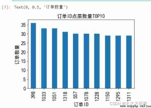
sort_counts['counts'][0:10].plot(kind='bar',fontsize=16)
plt.title(' Order ID Order quantity TOP10',fontsize='16')
plt.xlabel(' Order ID',fontsize='16')
plt.ylabel(' Order quantity ',fontsize='16')
#sort_counts['counts']
# Before the order quantity in August 10 name
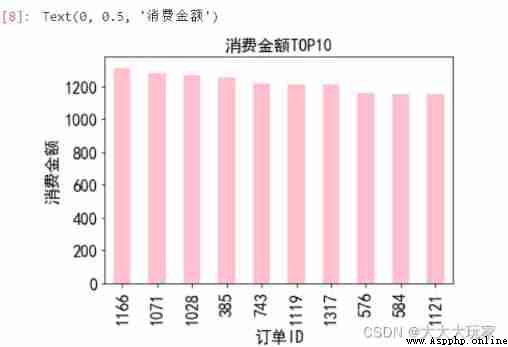
# That order costs the most
sort_tatal_amounts=Group_sum.sort_values(by='total_amounts',ascending=False)
sort_tatal_amounts['total_amounts'][:10].plot(kind='bar',fontsize='16',color='pink')
plt.title(' Consumption amount TOP10',fontsize='16')
plt.xlabel(' Order ID',fontsize='16')
plt.ylabel(' Consumption amount ',fontsize='16')
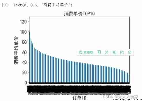
# Which order ID Average consumption is the most expensive
Group_sum['average']=Group_sum['total_amounts']/Group_sum['counts']
sort_average=Group_sum.sort_values(by='average',ascending=False)
sort_average['average'][:].plot(kind='bar',fontsize='16')
plt.title(' Consumption unit price TOP10',fontsize='16')
plt.xlabel(' Order ID',fontsize='16')
plt.ylabel(' Average unit price of consumption ',fontsize='16')
Analyze for time and date
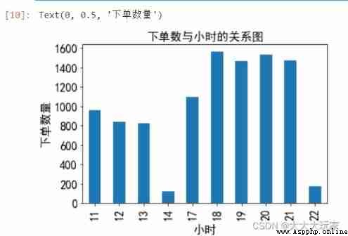
# What time of day , The number of orders is concentrated .
data['hourcount']=1 # New column , Use as counter
data['time']=pd.to_datetime(data['place_order_time'])# Convert time to date type for storage
data['hour']=data['time'].map(lambda x:x.hour)
gp_by_hour=data.groupby(by='hour').count()['hourcount']
gp_by_hour
gp_by_hour.plot(kind='bar',fontsize='16')
plt.title(' The relationship between the next singular number and the hour ',fontsize='16')
plt.xlabel(' Hours ',fontsize='16')
plt.ylabel(' Order quantity ',fontsize='16')
# The largest number of orders were placed on that day in August
data['daycount']=1
data['day']=data['time'].map(lambda x:x.day)# Resolution days
#data
gp_by_day=data.groupby(by='day').count()['daycount'] # Do not take out separately ['daycount'] Then each column will be counted
gp_by_day.plot(kind='bar',fontsize=16)
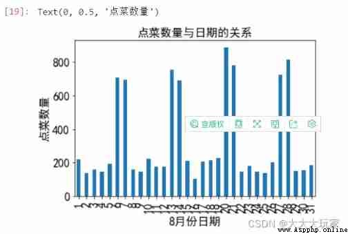
plt.title(' The relationship between order quantity and date ',fontsize='16')
plt.xlabel('8 Month date ',fontsize='16')
plt.ylabel(' Order quantity ',fontsize='16')
# You can sort , Take out the first five days of the largest order
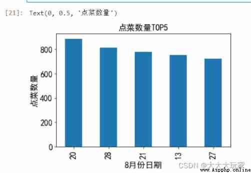
gp_sort_day=gp_by_day.sort_values(ascending=False)[:5]
gp_sort_day.plot(kind='bar',fontsize='16')
plt.title(' Order quantity TOP5',fontsize='16')
plt.xlabel('8 Month date ',fontsize='16')
plt.ylabel(' Order quantity ',fontsize='16')
# View the day of the week with the most people , Order the most meals , Map data to week
data['weekcount']=1# You can also use the previous counter , This will make it clearer
data['weekday']=data['time'].map(lambda x:x.weekday())
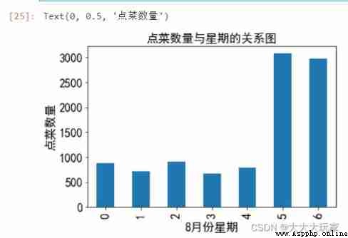
gp_by_weekday=data.groupby(by='weekday').count()['weekcount']
gp_by_weekday.plot(kind='bar',fontsize=16)
plt.title(' The relationship between order quantity and week ',fontsize='16')
plt.xlabel('8 Month week ',fontsize='16')
plt.ylabel(' Order quantity ',fontsize='16')
technology ( Data analysis in different dimensions )
For orders order_id:
 What dish is the most popular
The kind of order
Number of orders
The consumption amount is the largest
Average consumption is the most expensive
Analyze for time and date :
 A time when orders are concentrated
Which day has the largest number of orders
People like to eat on the day of the week
The day of the week has the largest number of diners
Technical point :
 Splicing data :pd.concat([ Column 1, Column 2, Column 3])
Statistics in groups ( Go and... In groups )
Sort , section TOP10
Analyze the trend and height of the histogram