In this job , You will use numpy Realize your first recurrent neural network .
Cyclic neural network (RNN) It is very effective in solving natural language processing and other sequential tasks , Because they have “ memory ”, You can read one input at a time x < t > x^{<t>} x<t>( For example, words ), And remember some information by activating the hidden layer that passes from one time step to the next / Context . This makes one-way RNN You can extract past information to process subsequent input . two-way RNN Then we can draw on the contextual information of the past and the future .
Symbol :
import numpy as np
import rnn_utils
Homework after this week , You will use RNN Making music . You will achieve the basic RNN It has the following structure . In this example , T x = T y T_x=T_y Tx=Ty.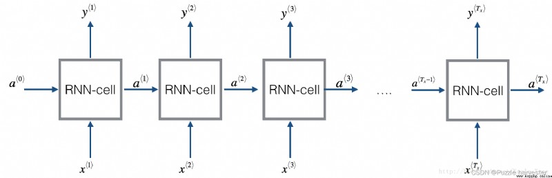
Realization RNN Methods :
step :
The recurrent neural network can be regarded as a single cell Duplication . You first have to calculate on a single time step . The following figure describes RNN Operation of a single time step of the unit .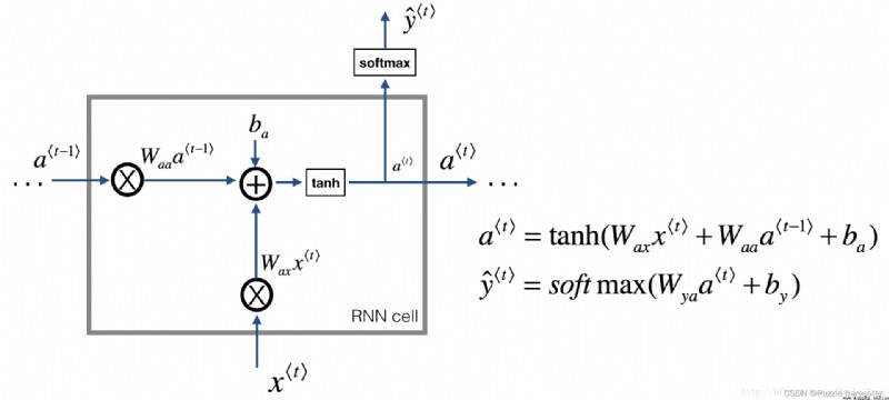
Basics RNN unit , take x < t > x^{<t>} x<t>( Current input ) and a < t − 1 > a^{<t-1>} a<t−1>( Include the current hidden state of past information ) As input , And the output a < t > a^{<t>} a<t> To the next RNN unit , Used to predict y < t > y^{<t>} y<t>.
practice : Realize the RNN unit .
explain :
softmax.We will be on m m m Examples are vectorized . therefore , x * t * x^{\langle t \rangle} x*t* Dimension will be ( n x , m ) (n_x,m) (nx,m), and a * t * a^{\langle t \rangle} a*t* Dimension will be ( n a , m ) (n_a,m) (na,m).
def rnn_cell_forward(xt, a_prev, parameters):
""" According to the figure 2 Realization RNN One step forward propagation of the unit Parameters : xt -- Time step "t" Input data , Dimension for (n_x, m) a_prev -- Time step "t - 1" The hidden state of , Dimension for (n_a, m) parameters -- Dictionaries , It includes the following : Wax -- matrix , Input multiplied by weight , Dimension for (n_a, n_x) Waa -- matrix , The hidden state is multiplied by the weight , Dimension for (n_a, n_a) Wya -- matrix , Hide the weight matrix related to the output , Dimension for (n_y, n_a) ba -- bias , Dimension for (n_a, 1) by -- bias , Hide the offset associated with the output , Dimension for (n_y, 1) return : a_next -- Next hidden state , Dimension for (n_a, m) yt_pred -- In time step “t” The forecast , Dimension for (n_y, m) cache -- Tuples required for back propagation , Contains (a_next, a_prev, xt, parameters) """
# from “parameters” To obtain parameters
Wax = parameters["Wax"]
Waa = parameters["Waa"]
Wya = parameters["Wya"]
ba = parameters["ba"]
by = parameters["by"]
# Use the above formula to calculate the next activation value
a_next = np.tanh(np.dot(Waa, a_prev) + np.dot(Wax, xt) + ba)
# Use the above formula to calculate the output of the current cell
yt_pred = rnn_utils.softmax(np.dot(Wya, a_next) + by)
# Save the values required for back propagation
cache = (a_next, a_prev, xt, parameters)
return a_next, yt_pred, cache
np.random.seed(1)
xt = np.random.randn(3,10)
a_prev = np.random.randn(5,10)
Waa = np.random.randn(5,5)
Wax = np.random.randn(5,3)
Wya = np.random.randn(2,5)
ba = np.random.randn(5,1)
by = np.random.randn(2,1)
parameters = {
"Waa": Waa, "Wax": Wax, "Wya": Wya, "ba": ba, "by": by}
a_next, yt_pred, cache = rnn_cell_forward(xt, a_prev, parameters)
print("a_next[4] = ", a_next[4])
print("a_next.shape = ", a_next.shape)
print("yt_pred[1] =", yt_pred[1])
print("yt_pred.shape = ", yt_pred.shape)
a_next[4] = [ 0.59584544 0.18141802 0.61311866 0.99808218 0.85016201 0.99980978
-0.18887155 0.99815551 0.6531151 0.82872037]
a_next.shape = (5, 10)
yt_pred[1] = [0.9888161 0.01682021 0.21140899 0.36817467 0.98988387 0.88945212
0.36920224 0.9966312 0.9982559 0.17746526]
yt_pred.shape = (2, 10)
You can take RNN As a repetition of the unit just built . If the input data sequence passes 10 Time steps , Will be copied RNN unit 10 Time . Each cell will replace the previous cell ( a * t − 1 * a^{\langle t-1 \rangle} a*t−1*) The hidden state of and the input data of the current time step ( x * t * x^{\langle t \rangle} x*t*) As input , And output the hidden state for this time step ( a * t * a^{\langle t \rangle} a*t*) And forecasting ( y * t * y^{\langle t \rangle} y*t*).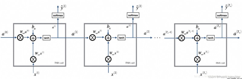
basic RNN. Input sequence x = ( x * 1 * , x * 2 * , . . . , x * T x * ) x = (x^{\langle 1 \rangle}, x^{\langle 2 \rangle}, ..., x^{\langle T_x \rangle}) x=(x*1*,x*2*,...,x*Tx*) perform T x T_x Tx Time steps . Network output y = ( y * 1 * , y * 2 * , . . . , y * T x * ) y = (y^{\langle 1 \rangle}, y^{\langle 2 \rangle}, ..., y^{\langle T_x \rangle}) y=(y*1*,y*2*,...,y*Tx*).
practice : The coding implements RNN Forward propagation of .
explain :
rnn_step_forward to update “ next ” Hide state and cache .def rnn_forward(x, a0, parameters):
""" According to the figure 3 Forward propagation of neural network Parameters : x -- All data entered , Dimension for (n_x, m, T_x) a0 -- Initialize hidden state , Dimension for (n_a, m) parameters -- Dictionaries , It includes the following : Wax -- matrix , Input multiplied by weight , Dimension for (n_a, n_x) Waa -- matrix , The hidden state is multiplied by the weight , Dimension for (n_a, n_a) Wya -- matrix , Hide the weight matrix related to the output , Dimension for (n_y, n_a) ba -- bias , Dimension for (n_a, 1) by -- bias , Hide the offset associated with the output , Dimension for (n_y, 1) return : a -- Hidden state of all time steps , Dimension for (n_a, m, T_x) y_pred -- Prediction of all time steps , Dimension for (n_y, m, T_x) caches -- Saved tuples for back propagation , Dimension for (【 List the type 】cache, x)) """
# initialization “caches”, It will contain all... In a list type cache
caches = []
# obtain x And Wya Dimension information of
n_x, m, T_x = x.shape
n_y, n_a = parameters["Wya"].shape
# Use 0 To initialize the “a” And “y”
a = np.zeros([n_a, m, T_x])
y_pred = np.zeros([n_y, m, T_x])
# initialization “next”
a_next = a0
# Traverse all time steps
for t in range(T_x):
## 1. Use rnn_cell_forward Function to update “next” Hidden state and cache.
a_next, yt_pred, cache = rnn_cell_forward(x[:, :, t], a_next, parameters)
## 2. Use a To preserve “next” Hidden state ( The first t ) A place .
a[:, :, t] = a_next
## 3. Use y To save the forecast .
y_pred[:, :, t] = yt_pred
## 4. hold cache Save to “caches” In the list .
caches.append(cache)
# Save the parameters required for back propagation
caches = (caches, x)
return a, y_pred, caches
np.random.seed(1)
x = np.random.randn(3,10,4)
a0 = np.random.randn(5,10)
Waa = np.random.randn(5,5)
Wax = np.random.randn(5,3)
Wya = np.random.randn(2,5)
ba = np.random.randn(5,1)
by = np.random.randn(2,1)
parameters = {
"Waa": Waa, "Wax": Wax, "Wya": Wya, "ba": ba, "by": by}
a, y_pred, caches = rnn_forward(x, a0, parameters)
print("a[4][1] = ", a[4][1])
print("a.shape = ", a.shape)
print("y_pred[1][3] =", y_pred[1][3])
print("y_pred.shape = ", y_pred.shape)
print("caches[1][1][3] =", caches[1][1][3])
print("len(caches) = ", len(caches))
a[4][1] = [-0.99999375 0.77911235 -0.99861469 -0.99833267]
a.shape = (5, 10, 4)
y_pred[1][3] = [0.79560373 0.86224861 0.11118257 0.81515947]
y_pred.shape = (2, 10, 4)
caches[1][1][3] = [-1.1425182 -0.34934272 -0.20889423 0.58662319]
len(caches) = 2
Nice! You have realized the forward propagation of the recurrent neural network from scratch . For some applications , This is good enough , But we will encounter the problem of gradient disappearance . therefore , When each output y * t * y^{\langle t \rangle} y*t* The main use of "local" It performs best in context estimation ( That is, from the input x * t ′ * x^{\langle t' \rangle} x*t′* Information about , among t ′ t' t′ It's distance t t t Closer ).
thereinafter , You will build a more complex LSTM Model , This model is more suitable for solving the gradual disappearance of gradients .LSTM Will be able to better remember a piece of information and save it for many time steps .
The image below shows LSTM Operation of the unit .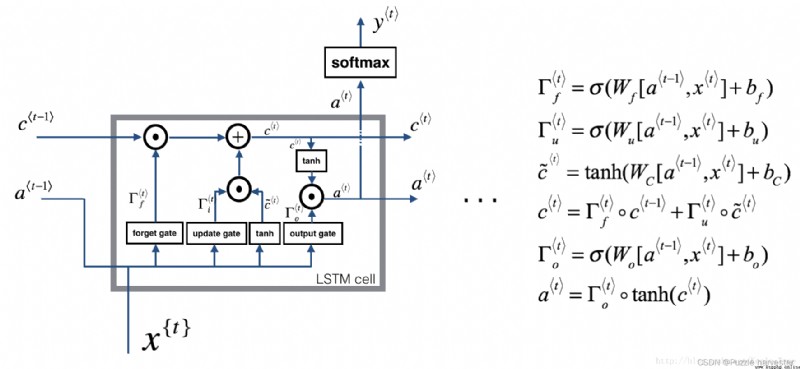
LSTM unit , This will be tracked and updated at each time step “ Unit status ” Or stored variables c * t * c^{\langle t \rangle} c*t*, And a * t * a^{\langle t \rangle} a*t* Different .
With the above RNN The example is similar to , You will start with a single time step LSTM unit . then , You can start your for Loop internal iteration calls it , So that it has T x T_x Tx Input of time step .
For the sake of illustration , Suppose we are reading words in a text , And hope to use LSTM Track grammatical structure , For example, is the subject singular or plural . If the subject changes from singular to plural , We need to find a way to get rid of the previously stored orders / Memory value of complex state . stay LSTM in , Forgetting gate can realize times operation :
Γ f * t * = σ ( W f [ a * t − 1 * , x * t * ] + b f ) (1) \Gamma_f^{\langle t \rangle} = \sigma(W_f[a^{\langle t-1 \rangle}, x^{\langle t \rangle}] + b_f)\tag{1} Γf*t*=σ(Wf[a*t−1*,x*t*]+bf)(1)
ad locum , W f W_f Wf It is the weight that controls the behavior of forgetting gate . We will [ a * t − 1 * , x * t * ] [a^{\langle t-1 \rangle}, x^{\langle t \rangle}] [a*t−1*,x*t*] Connect , And then multiplied by the W f W_f Wf. The above equation makes the vector Γ f * t * \Gamma_f^{\langle t \rangle} Γf*t* The value is between 0 To 1 Between . The forgetting gate vector multiplies the previous cell state on an element by element basis c * t − 1 * c^{\langle t-1 \rangle} c*t−1*. therefore , If Γ f * t * \Gamma_f^{\langle t \rangle} Γf*t* One of the values of is 0( Or close to 0), said LSTM It should be removed c * t − 1 * c^{\langle t-1 \rangle} c*t−1* Part of the information in the component ( for example , Singular theme ), If one of the values is 1, Then it will retain the information .
Once we forget that the subject in question is singular , We need to find a way to update it , To reflect that the new subject is now plural . This is the formula for updating the door :
Γ u * t * = σ ( W u [ a * t − 1 * , x { t } ] + b u ) (2) \Gamma_u^{\langle t \rangle} = \sigma(W_u[a^{\langle t-1 \rangle}, x^{\{t\}}] + b_u)\tag{2} Γu*t*=σ(Wu[a*t−1*,x{ t}]+bu)(2)
Similar to the forgetting door , ad locum Γ u * t * \Gamma_u^{\langle t \rangle} Γu*t* It is also worth 0 To 1 The vector between . This will c ~ * t * \tilde{c}^{\langle t \rangle} c~*t* Multiply by each element c * t * c^{\langle t \rangle} c*t*.
To update the new body , We need to create a new number vector , You can add it to the previous cell state . The equation we use is :
c ~ * t * = tanh ( W c [ a * t − 1 * , x * t * ] + b c ) (3) \tilde{c}^{\langle t \rangle} = \tanh(W_c[a^{\langle t-1 \rangle}, x^{\langle t \rangle}] + b_c)\tag{3} c~*t*=tanh(Wc[a*t−1*,x*t*]+bc)(3)
Last , The new unit status is :
c * t * = Γ f * t * ∗ c * t − 1 * + Γ u * t * ∗ c ~ * t * (4) c^{\langle t \rangle} = \Gamma_f^{\langle t \rangle}* c^{\langle t-1 \rangle} + \Gamma_u^{\langle t \rangle} *\tilde{c}^{\langle t \rangle} \tag{4} c*t*=Γf*t*∗c*t−1*+Γu*t*∗c~*t*(4)
To determine which outputs we will use , We will use the following two formulas :
Γ o * t * = σ ( W o [ a * t − 1 * , x * t * ] + b o ) (5) \Gamma_o^{\langle t \rangle}= \sigma(W_o[a^{\langle t-1 \rangle}, x^{\langle t \rangle}] + b_o)\tag{5} Γo*t*=σ(Wo[a*t−1*,x*t*]+bo)(5)
a * t * = Γ o * t * ∗ tanh ( c * t * ) (6) a^{\langle t \rangle} = \Gamma_o^{\langle t \rangle}* \tanh(c^{\langle t \rangle})\tag{6} a*t*=Γo*t*∗tanh(c*t*)(6)
In the equation 5 in , You decide to use sigmoid Output function ; In the equation 6 in , Multiply it by the previous state tanh.
practice : Realize the LSTM unit .
explain :
sigmoid() and np.tanh().sigmoid().def lstm_cell_forward(xt, a_prev, c_prev, parameters):
""" According to the figure 4 Achieve one LSTM Forward propagation of the unit . Parameters : xt -- In time step “t” Input data , Dimension for (n_x, m) a_prev -- Last time step “t-1” The hidden state of , Dimension for (n_a, m) c_prev -- Last time step “t-1” My memory state , Dimension for (n_a, m) parameters -- Dictionary type variables , Contains : Wf -- Forget the weight of the door , Dimension for (n_a, n_a + n_x) bf -- Forget the offset of the door , Dimension for (n_a, 1) Wi -- Update the weight of the door , Dimension for (n_a, n_a + n_x) bi -- Update the offset of the door , Dimension for (n_a, 1) Wc -- first “tanh” A weight , Dimension for (n_a, n_a + n_x) bc -- first “tanh” The offset of , Dimension for (n_a, n_a + n_x) Wo -- The weight of the output gate , Dimension for (n_a, n_a + n_x) bo -- Output gate offset , Dimension for (n_a, 1) Wy -- Hide the weights related to the state and output , Dimension for (n_y, n_a) by -- Hide the offset associated with the output , Dimension for (n_y, 1) return : a_next -- Next hidden state , Dimension for (n_a, m) c_next -- Next memory state , Dimension for (n_a, m) yt_pred -- In time step “t” The forecast , Dimension for (n_y, m) cache -- Contains the parameters required for back propagation , Contains (a_next, c_next, a_prev, c_prev, xt, parameters) Be careful : ft/it/ot Indicates forgetting / to update / Output gate ,cct Indicates the candidate value (c tilda),c Indicates the memory value . """
# from “parameters” Get relevant values from
Wf = parameters["Wf"]
bf = parameters["bf"]
Wi = parameters["Wi"]
bi = parameters["bi"]
Wc = parameters["Wc"]
bc = parameters["bc"]
Wo = parameters["Wo"]
bo = parameters["bo"]
Wy = parameters["Wy"]
by = parameters["by"]
# obtain xt And Wy Dimension information of
n_x, m = xt.shape
n_y, n_a = Wy.shape
# 1. Connect a_prev And xt
contact = np.zeros([n_a + n_x, m])
contact[: n_a, :] = a_prev
contact[n_a :, :] = xt
# 2. According to the formula ft、it、cct、c_next、ot、a_next
## Oblivion gate , The formula 1
ft = rnn_utils.sigmoid(np.dot(Wf, contact) + bf)
## Update door , The formula 2
it = rnn_utils.sigmoid(np.dot(Wi, contact) + bi)
## Update unit , The formula 3
cct = np.tanh(np.dot(Wc, contact) + bc)
## Update unit , The formula 4
#c_next = np.multiply(ft, c_prev) + np.multiply(it, cct)
c_next = ft * c_prev + it * cct
## Output gate , The formula 5
ot = rnn_utils.sigmoid(np.dot(Wo, contact) + bo)
## Output gate , The formula 6
#a_next = np.multiply(ot, np.tan(c_next))
a_next = ot * np.tanh(c_next)
# 3. Calculation LSTM The predicted value of the unit
yt_pred = rnn_utils.softmax(np.dot(Wy, a_next) + by)
# Save contains the parameters required for back propagation
cache = (a_next, c_next, a_prev, c_prev, ft, it, cct, ot, xt, parameters)
return a_next, c_next, yt_pred, cache
np.random.seed(1)
xt = np.random.randn(3,10)
a_prev = np.random.randn(5,10)
c_prev = np.random.randn(5,10)
Wf = np.random.randn(5, 5+3)
bf = np.random.randn(5,1)
Wi = np.random.randn(5, 5+3)
bi = np.random.randn(5,1)
Wo = np.random.randn(5, 5+3)
bo = np.random.randn(5,1)
Wc = np.random.randn(5, 5+3)
bc = np.random.randn(5,1)
Wy = np.random.randn(2,5)
by = np.random.randn(2,1)
parameters = {
"Wf": Wf, "Wi": Wi, "Wo": Wo, "Wc": Wc, "Wy": Wy, "bf": bf, "bi": bi, "bo": bo, "bc": bc, "by": by}
a_next, c_next, yt, cache = lstm_cell_forward(xt, a_prev, c_prev, parameters)
print("a_next[4] = ", a_next[4])
print("a_next.shape = ", c_next.shape)
print("c_next[2] = ", c_next[2])
print("c_next.shape = ", c_next.shape)
print("yt[1] =", yt[1])
print("yt.shape = ", yt.shape)
print("cache[1][3] =", cache[1][3])
print("len(cache) = ", len(cache))
a_next[4] = [-0.66408471 0.0036921 0.02088357 0.22834167 -0.85575339 0.00138482
0.76566531 0.34631421 -0.00215674 0.43827275]
a_next.shape = (5, 10)
c_next[2] = [ 0.63267805 1.00570849 0.35504474 0.20690913 -1.64566718 0.11832942
0.76449811 -0.0981561 -0.74348425 -0.26810932]
c_next.shape = (5, 10)
yt[1] = [0.79913913 0.15986619 0.22412122 0.15606108 0.97057211 0.31146381
0.00943007 0.12666353 0.39380172 0.07828381]
yt.shape = (2, 10)
cache[1][3] = [-0.16263996 1.03729328 0.72938082 -0.54101719 0.02752074 -0.30821874
0.07651101 -1.03752894 1.41219977 -0.37647422]
len(cache) = 10
Now that you have achieved LSTM One step of , You can use it now for The cycle is T x T_x Tx Iterate over this on the input sequence .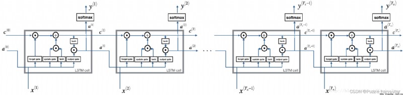
practice : Realization lstm_forward() In the T x T_x Tx Run on time steps LSTM.
Be careful : c * 0 * c^{\langle 0 \rangle} c*0* Initialize with zero .
def lstm_forward(x, a0, parameters):
""" According to the figure 5 To achieve LSTM A cyclic neural network composed of units Parameters : x -- Input data for all time steps , Dimension for (n_x, m, T_x) a0 -- Initialize hidden state , Dimension for (n_a, m) parameters -- python Dictionaries , Contains the following parameters : Wf -- Forget the weight of the door , Dimension for (n_a, n_a + n_x) bf -- Forget the offset of the door , Dimension for (n_a, 1) Wi -- Update the weight of the door , Dimension for (n_a, n_a + n_x) bi -- Update the offset of the door , Dimension for (n_a, 1) Wc -- first “tanh” A weight , Dimension for (n_a, n_a + n_x) bc -- first “tanh” The offset of , Dimension for (n_a, n_a + n_x) Wo -- The weight of the output gate , Dimension for (n_a, n_a + n_x) bo -- Output gate offset , Dimension for (n_a, 1) Wy -- Hide the weights related to the state and output , Dimension for (n_y, n_a) by -- Hide the offset associated with the output , Dimension for (n_y, 1) return : a -- Hidden state of all time steps , Dimension for (n_a, m, T_x) y -- Predicted values for all time steps , Dimension for (n_y, m, T_x) caches -- Saved tuples for back propagation , Dimension for (【 List the type 】cache, x)) """
# initialization “caches”
caches = []
# obtain xt And Wy Dimension information of
n_x, m, T_x = x.shape
n_y, n_a = parameters["Wy"].shape
# Use 0 To initialize the “a”、“c”、“y”
a = np.zeros([n_a, m, T_x])
c = np.zeros([n_a, m, T_x])
y = np.zeros([n_y, m, T_x])
# initialization “a_next”、“c_next”
a_next = a0
c_next = np.zeros([n_a, m])
# Go through all the time steps
for t in range(T_x):
# Update the next hidden state , Next memory state , Calculate the predicted value , obtain cache
a_next, c_next, yt_pred, cache = lstm_cell_forward(x[:,:,t], a_next, c_next, parameters)
# Save the new next hidden state to the variable a in
a[:, :, t] = a_next
# Save the predicted value to the variable y in
y[:, :, t] = yt_pred
# Save the next cell state to the variable c in
c[:, :, t] = c_next
# hold cache Add to caches in
caches.append(cache)
# Save the parameters required for back propagation
caches = (caches, x)
return a, y, c, caches
np.random.seed(1)
x = np.random.randn(3,10,7)
a0 = np.random.randn(5,10)
Wf = np.random.randn(5, 5+3)
bf = np.random.randn(5,1)
Wi = np.random.randn(5, 5+3)
bi = np.random.randn(5,1)
Wo = np.random.randn(5, 5+3)
bo = np.random.randn(5,1)
Wc = np.random.randn(5, 5+3)
bc = np.random.randn(5,1)
Wy = np.random.randn(2,5)
by = np.random.randn(2,1)
parameters = {
"Wf": Wf, "Wi": Wi, "Wo": Wo, "Wc": Wc, "Wy": Wy, "bf": bf, "bi": bi, "bo": bo, "bc": bc, "by": by}
a, y, c, caches = lstm_forward(x, a0, parameters)
print("a[4][3][6] = ", a[4][3][6])
print("a.shape = ", a.shape)
print("y[1][4][3] =", y[1][4][3])
print("y.shape = ", y.shape)
print("caches[1][1[1]] =", caches[1][1][1])
print("c[1][2][1]", c[1][2][1])
print("len(caches) = ", len(caches))
a[4][3][6] = 0.17211776753291672
a.shape = (5, 10, 7)
y[1][4][3] = 0.9508734618501101
y.shape = (2, 10, 7)
caches[1][1[1]] = [ 0.82797464 0.23009474 0.76201118 -0.22232814 -0.20075807 0.18656139
0.41005165]
c[1][2][1] -0.8555449167181981
len(caches) = 2
In the framework of modern deep learning , You just need to achieve forward propagation , The framework will handle back propagation , Therefore, most deep learning engineers do not need to pay attention to the details of back-propagation . however , If you are an expert in calculus and want to check RNN Details of back propagation in , You can learn the rest of this notebook .
In earlier courses , When you implement a simple ( All of the connection ) When neural networks , You use back propagation to calculate the derivative of the loss used to update the parameter . Again , In a recurrent neural network , You can calculate the derivative of the loss to update the parameters . The back propagation equation is very complex , We didn't export them in the lecture . however , We will briefly introduce them below .
We will start from the basic calculation RNN The back propagation of the unit begins .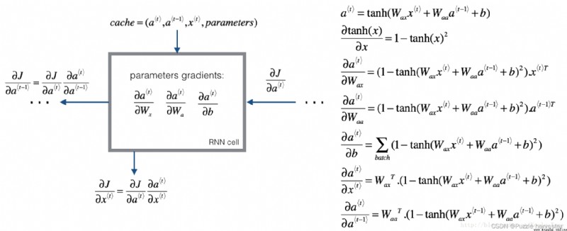
Just like in a fully connected neural network , Loss function J J J The derivative of follows the chain rule at RNN Calculate back propagation . Chain rules are also used to calculate ( ∂ J ∂ W a x , ∂ J ∂ W a a , ∂ J ∂ b ) (\frac{\partial J}{\partial W_{ax}},\frac{\partial J}{\partial W_{aa}},\frac{\partial J}{\partial b}) (∂Wax∂J,∂Waa∂J,∂b∂J) Update parameters ( W a x , W a a , b a ) (W_{ax}, W_{aa}, b_a) (Wax,Waa,ba).
To calculate rnn_cell_backward, You need to calculate the following equation . Exporting them manually is a good exercise .
tanh \tanh tanh The derivative of is 1 − tanh ( x ) 2 1-\tanh(x)^2 1−tanh(x)2. You can here Find complete proof in . Please note that :$ \text{sech}(x)^2 = 1 - \tanh(x)^2$
Again , about ∂ a * t * ∂ W a x , ∂ a * t * ∂ W a a , ∂ a * t * ∂ b \frac{ \partial a^{\langle t \rangle} } {\partial W_{ax}}, \frac{ \partial a^{\langle t \rangle} } {\partial W_{aa}}, \frac{ \partial a^{\langle t \rangle} } {\partial b} ∂Wax∂a*t*,∂Waa∂a*t*,∂b∂a*t*, tanh ( u ) \tanh(u) tanh(u) Derivative is ( 1 − tanh ( u ) 2 ) d u (1-\tanh(u)^2)du (1−tanh(u)2)du.
The last two equations follow the same rules , And use tanh \tanh tanh Derivative derivation . Please note that , This arrangement is to obtain the same dimensions to facilitate matching .
def rnn_cell_backward(da_next, cache):
""" Implement the basic RNN Single step back propagation of unit Parameters : da_next -- The gradient of the loss of the next hidden state . cache -- Dictionary type ,rnn_step_forward() Output return : gradients -- Dictionaries , Contains the following parameters : dx -- Gradient of input data , Dimension for (n_x, m) da_prev -- The hidden state of the previous hidden layer , Dimension for (n_a, m) dWax -- The gradient of the weight entered into the hidden state , Dimension for (n_a, n_x) dWaa -- Gradient of weight from hidden state to hidden state , Dimension for (n_a, n_a) dba -- The gradient of the offset vector , Dimension for (n_a, 1) """
# obtain cache Value
a_next, a_prev, xt, parameters = cache
# from parameters Get parameters in
Wax = parameters["Wax"]
Waa = parameters["Waa"]
Wya = parameters["Wya"]
ba = parameters["ba"]
by = parameters["by"]
# Calculation tanh be relative to a_next Gradient of .
dtanh = (1 - np.square(a_next)) * da_next
# Calculate about Wax The gradient of loss
dxt = np.dot(Wax.T,dtanh)
dWax = np.dot(dtanh, xt.T)
# Calculate about Waa The gradient of loss
da_prev = np.dot(Waa.T,dtanh)
dWaa = np.dot(dtanh, a_prev.T)
# Calculate about b The gradient of loss
dba = np.sum(dtanh, keepdims=True, axis=-1)
# Save these gradients into the dictionary
gradients = {
"dxt": dxt, "da_prev": da_prev, "dWax": dWax, "dWaa": dWaa, "dba": dba}
return gradients
np.random.seed(1)
xt = np.random.randn(3,10)
a_prev = np.random.randn(5,10)
Wax = np.random.randn(5,3)
Waa = np.random.randn(5,5)
Wya = np.random.randn(2,5)
b = np.random.randn(5,1)
by = np.random.randn(2,1)
parameters = {
"Wax": Wax, "Waa": Waa, "Wya": Wya, "ba": ba, "by": by}
a_next, yt, cache = rnn_cell_forward(xt, a_prev, parameters)
da_next = np.random.randn(5,10)
gradients = rnn_cell_backward(da_next, cache)
print("gradients[\"dxt\"][1][2] =", gradients["dxt"][1][2])
print("gradients[\"dxt\"].shape =", gradients["dxt"].shape)
print("gradients[\"da_prev\"][2][3] =", gradients["da_prev"][2][3])
print("gradients[\"da_prev\"].shape =", gradients["da_prev"].shape)
print("gradients[\"dWax\"][3][1] =", gradients["dWax"][3][1])
print("gradients[\"dWax\"].shape =", gradients["dWax"].shape)
print("gradients[\"dWaa\"][1][2] =", gradients["dWaa"][1][2])
print("gradients[\"dWaa\"].shape =", gradients["dWaa"].shape)
print("gradients[\"dba\"][4] =", gradients["dba"][4])
print("gradients[\"dba\"].shape =", gradients["dba"].shape)
gradients["dxt"][1][2] = -0.4605641030588796
gradients["dxt"].shape = (3, 10)
gradients["da_prev"][2][3] = 0.08429686538067718
gradients["da_prev"].shape = (5, 10)
gradients["dWax"][3][1] = 0.3930818739219304
gradients["dWax"].shape = (5, 3)
gradients["dWaa"][1][2] = -0.2848395578696067
gradients["dWaa"].shape = (5, 5)
gradients["dba"][4] = [0.80517166]
gradients["dba"].shape = (5, 1)
At each time step t t t The upper calculation is relative to a * t * a^{\langle t \rangle} a*t* The loss gradient of is very useful , Because it helps to propagate the gradient back to the previous RNN unit . So , You need to go through all the time steps from scratch , And in every step , Increase the total d b a db_a dba, d W a a dW_{aa} dWaa, d W a x dW_{ax} dWax And store d x dx dx.
explain :
Realization rnn_backward function . First initialize the return variable with zero , Then loop through all time steps , At the same time, call at each time step rnn_cell_backward, Update other variables accordingly .
def rnn_backward(da, caches):
""" Implement... On the whole input data sequence RNN Back propagation of Parameters : da -- Gradients of all hidden states , Dimension for (n_a, m, T_x) caches -- Tuples containing forward propagating information return : gradients -- A dictionary containing gradients : dx -- About the gradient of input data , Dimension for (n_x, m, T_x) da0 -- On the gradient of initializing the hidden state , Dimension for (n_a, m) dWax -- About the gradient of input weight , Dimension for (n_a, n_x) dWaa -- On the gradient of the weight of the hidden state , Dimension for (n_a, n_a) dba -- About the gradient of bias , Dimension for (n_a, 1) """
# from caches Get the first cache(t=1) Value
caches, x = caches
a1, a0, x1, parameters = caches[0]
# obtain da And x1 Dimension information of
n_a, m, T_x = da.shape
n_x, m = x1.shape
# Initialization gradient
dx = np.zeros([n_x, m, T_x])
dWax = np.zeros([n_a, n_x])
dWaa = np.zeros([n_a, n_a])
dba = np.zeros([n_a, 1])
da0 = np.zeros([n_a, m])
da_prevt = np.zeros([n_a, m])
# Process all time steps
for t in reversed(range(T_x)):
# Calculate the time step “t” The gradient of time
gradients = rnn_cell_backward(da[:, :, t] + da_prevt, caches[t])
# Take the derivative from the gradient
dxt, da_prevt, dWaxt, dWaat, dbat = gradients["dxt"], gradients["da_prev"], gradients["dWax"], gradients["dWaa"], gradients["dba"]
# Through the time step t Add their derivatives to increase the parameters about the global derivatives
dx[:, :, t] = dxt
dWax += dWaxt
dWaa += dWaat
dba += dbat
# take da0 Set to a Gradient of , The gradient has been back propagated through all time steps
da0 = da_prevt
# Save these gradients into the dictionary
gradients = {
"dx": dx, "da0": da0, "dWax": dWax, "dWaa": dWaa,"dba": dba}
return gradients
np.random.seed(1)
x = np.random.randn(3,10,4)
a0 = np.random.randn(5,10)
Wax = np.random.randn(5,3)
Waa = np.random.randn(5,5)
Wya = np.random.randn(2,5)
ba = np.random.randn(5,1)
by = np.random.randn(2,1)
parameters = {
"Wax": Wax, "Waa": Waa, "Wya": Wya, "ba": ba, "by": by}
a, y, caches = rnn_forward(x, a0, parameters)
da = np.random.randn(5, 10, 4)
gradients = rnn_backward(da, caches)
print("gradients[\"dx\"][1][2] =", gradients["dx"][1][2])
print("gradients[\"dx\"].shape =", gradients["dx"].shape)
print("gradients[\"da0\"][2][3] =", gradients["da0"][2][3])
print("gradients[\"da0\"].shape =", gradients["da0"].shape)
print("gradients[\"dWax\"][3][1] =", gradients["dWax"][3][1])
print("gradients[\"dWax\"].shape =", gradients["dWax"].shape)
print("gradients[\"dWaa\"][1][2] =", gradients["dWaa"][1][2])
print("gradients[\"dWaa\"].shape =", gradients["dWaa"].shape)
print("gradients[\"dba\"][4] =", gradients["dba"][4])
print("gradients[\"dba\"].shape =", gradients["dba"].shape)
gradients["dx"][1][2] = [-2.07101689 -0.59255627 0.02466855 0.01483317]
gradients["dx"].shape = (3, 10, 4)
gradients["da0"][2][3] = -0.31494237512664996
gradients["da0"].shape = (5, 10)
gradients["dWax"][3][1] = 11.264104496527777
gradients["dWax"].shape = (5, 3)
gradients["dWaa"][1][2] = 2.3033331265798935
gradients["dWaa"].shape = (5, 5)
gradients["dba"][4] = [-0.74747722]
gradients["dba"].shape = (5, 1)
LSTM Back propagation is much more complicated than forward propagation . We provide you with LSTM All equations of back propagation .( If you like calculus practice , You can try to calculate from scratch )
d Γ o * t * = d a n e x t ∗ tanh ( c n e x t ) ∗ Γ o * t * ∗ ( 1 − Γ o * t * ) (7) d \Gamma_o^{\langle t \rangle} = da_{next}*\tanh(c_{next}) * \Gamma_o^{\langle t \rangle}*(1-\Gamma_o^{\langle t \rangle})\tag{7} dΓo*t*=danext∗tanh(cnext)∗Γo*t*∗(1−Γo*t*)(7)
d c ~ * t * = ( d c n e x t ∗ Γ u * t * + Γ o * t * ( 1 − tanh ( c n e x t ) 2 ) ∗ i t ∗ d a n e x t ∗ c ~ * t * ) ∗ ( 1 − tanh ( c ~ ) 2 ) (8) d\tilde c^{\langle t \rangle} = (dc_{next}*\Gamma_u^{\langle t \rangle}+ \Gamma_o^{\langle t \rangle} (1-\tanh(c_{next})^2) * i_t * da_{next} * \tilde c^{\langle t \rangle}) * (1-\tanh(\tilde c)^2) \tag{8} dc~*t*=(dcnext∗Γu*t*+Γo*t*(1−tanh(cnext)2)∗it∗danext∗c~*t*)∗(1−tanh(c~)2)(8)
d Γ u * t * = ( d c n e x t ∗ c ~ * t * + Γ o * t * ( 1 − tanh ( c n e x t ) 2 ) ∗ c ~ * t * ∗ d a n e x t ) ∗ Γ u * t * ∗ ( 1 − Γ u * t * ) (9) d\Gamma_u^{\langle t \rangle} = (dc_{next}*\tilde c^{\langle t \rangle} + \Gamma_o^{\langle t \rangle} (1-\tanh(c_{next})^2) * \tilde c^{\langle t \rangle} * da_{next})*\Gamma_u^{\langle t \rangle}*(1-\Gamma_u^{\langle t \rangle})\tag{9} dΓu*t*=(dcnext∗c~*t*+Γo*t*(1−tanh(cnext)2)∗c~*t*∗danext)∗Γu*t*∗(1−Γu*t*)(9)
d Γ f * t * = ( d c n e x t ∗ c ~ p r e v + Γ o * t * ( 1 − tanh ( c n e x t ) 2 ) ∗ c p r e v ∗ d a n e x t ) ∗ Γ f * t * ∗ ( 1 − Γ f * t * ) (10) d\Gamma_f^{\langle t \rangle} = (dc_{next}*\tilde c_{prev} + \Gamma_o^{\langle t \rangle} (1-\tanh(c_{next})^2) * c_{prev} * da_{next})*\Gamma_f^{\langle t \rangle}*(1-\Gamma_f^{\langle t \rangle})\tag{10} dΓf*t*=(dcnext∗c~prev+Γo*t*(1−tanh(cnext)2)∗cprev∗danext)∗Γf*t*∗(1−Γf*t*)(10)
d W f = d Γ f * t * ∗ ( a p r e v x t ) T (11) dW_f = d\Gamma_f^{\langle t \rangle} * \begin{pmatrix} a_{prev} \\ x_t\end{pmatrix}^T \tag{11} dWf=dΓf*t*∗(aprevxt)T(11)
d W u = d Γ u * t * ∗ ( a p r e v x t ) T (12) dW_u = d\Gamma_u^{\langle t \rangle} * \begin{pmatrix} a_{prev} \\ x_t\end{pmatrix}^T \tag{12} dWu=dΓu*t*∗(aprevxt)T(12)
d W c = d c ~ * t * ∗ ( a p r e v x t ) T (13) dW_c = d\tilde c^{\langle t \rangle} * \begin{pmatrix} a_{prev} \\ x_t\end{pmatrix}^T \tag{13} dWc=dc~*t*∗(aprevxt)T(13)
d W o = d Γ o * t * ∗ ( a p r e v x t ) T (14) dW_o = d\Gamma_o^{\langle t \rangle} * \begin{pmatrix} a_{prev} \\ x_t\end{pmatrix}^T \tag{14} dWo=dΓo*t*∗(aprevxt)T(14)
To calculate d b f , d b u , d b c , d b o db_f, db_u, db_c, db_o dbf,dbu,dbc,dbo, You just need to d Γ f * t * , d Γ u * t * , d c ~ * t * , d Γ o * t * d\Gamma_f^{\langle t \rangle}, d\Gamma_u^{\langle t \rangle}, d\tilde c^{\langle t \rangle}, d\Gamma_o^{\langle t \rangle} dΓf*t*,dΓu*t*,dc~*t*,dΓo*t* The level of (axis=1) Sum separately on the axis . Be careful , You should have keep_dims = True Options .
Last , You will aim at the previous hidden state , The previous memory state and input calculate the derivative .
d a p r e v = W f T ∗ d Γ f * t * + W u T ∗ d Γ u * t * + W c T ∗ d c ~ * t * + W o T ∗ d Γ o * t * (15) da_{prev} = W_f^T*d\Gamma_f^{\langle t \rangle} + W_u^T * d\Gamma_u^{\langle t \rangle}+ W_c^T * d\tilde c^{\langle t \rangle} + W_o^T * d\Gamma_o^{\langle t \rangle} \tag{15} daprev=WfT∗dΓf*t*+WuT∗dΓu*t*+WcT∗dc~*t*+WoT∗dΓo*t*(15)
ad locum , equation 13 The weight of is n_a individual ( namely W f = W f [ : , : n a ] W_f = W_f[:,:n_a] Wf=Wf[:,:na] etc. …)
d c p r e v = d c n e x t Γ f * t * + Γ o * t * ∗ ( 1 − tanh ( c n e x t ) 2 ) ∗ Γ f * t * ∗ d a n e x t (16) dc_{prev} = dc_{next}\Gamma_f^{\langle t \rangle} + \Gamma_o^{\langle t \rangle} * (1- \tanh(c_{next})^2)*\Gamma_f^{\langle t \rangle}*da_{next} \tag{16} dcprev=dcnextΓf*t*+Γo*t*∗(1−tanh(cnext)2)∗Γf*t*∗danext(16)
d x * t * = W f T ∗ d Γ f * t * + W u T ∗ d Γ u * t * + W c T ∗ d c ~ t + W o T ∗ d Γ o * t * (17) dx^{\langle t \rangle} = W_f^T*d\Gamma_f^{\langle t \rangle} + W_u^T * d\Gamma_u^{\langle t \rangle}+ W_c^T * d\tilde c_t + W_o^T * d\Gamma_o^{\langle t \rangle}\tag{17} dx*t*=WfT∗dΓf*t*+WuT∗dΓu*t*+WcT∗dc~t+WoT∗dΓo*t*(17)
Where the equation 15 The weight of is from n_a To the end ( namely W f = W f [ : , n a : ] W_f = W_f[:,n_a:] Wf=Wf[:,na:] etc. …)
practice : By implementing the following equation lstm_cell_backward.
def lstm_cell_backward(da_next, dc_next, cache):
""" Realization LSTM One step back propagation Parameters : da_next -- The gradient of the next hidden state , Dimension for (n_a, m) dc_next -- The next state of the gradient element , Dimension for (n_a, m) cache -- Some parameters from forward propagation return : gradients -- A dictionary containing gradient information : dxt -- Gradient of input data , Dimension for (n_x, m) da_prev -- The gradient of the previous hidden state , Dimension for (n_a, m) dc_prev -- The gradient of pre memory state , Dimension for (n_a, m, T_x) dWf -- The gradient of the weight of the forgetting gate , Dimension for (n_a, n_a + n_x) dbf -- The gradient of the bias of the forgetting gate , Dimension for (n_a, 1) dWi -- Update the gradient of the weight of the door , Dimension for (n_a, n_a + n_x) dbi -- Update the gradient of the offset of the door , Dimension for (n_a, 1) dWc -- first “tanh” The gradient of the weight of , Dimension for (n_a, n_a + n_x) dbc -- first “tanh” The gradient of the offset , Dimension for (n_a, n_a + n_x) dWo -- The gradient of the weight of the output gate , Dimension for (n_a, n_a + n_x) dbo -- The gradient of the bias of the output gate , Dimension for (n_a, 1) """
# from cache For information
(a_next, c_next, a_prev, c_prev, ft, it, cct, ot, xt, parameters) = cache
# obtain xt And a_next Dimension information of
n_x, m = xt.shape
n_a, m = a_next.shape
# According to the formula 7-10 To calculate the derivative of the gate
dot = da_next * np.tanh(c_next) * ot * (1 - ot)
dcct = (dc_next * it + ot * (1 - np.square(np.tanh(c_next))) * it * da_next) * (1 - np.square(cct))
dit = (dc_next * cct + ot * (1 - np.square(np.tanh(c_next))) * cct * da_next) * it * (1 - it)
dft = (dc_next * c_prev + ot * (1 - np.square(np.tanh(c_next))) * c_prev * da_next) * ft * (1 - ft)
# According to the formula 11-14 Calculate the derivative of the parameter
concat = np.concatenate((a_prev, xt), axis=0).T
dWf = np.dot(dft, concat)
dWi = np.dot(dit, concat)
dWc = np.dot(dcct, concat)
dWo = np.dot(dot, concat)
dbf = np.sum(dft,axis=1,keepdims=True)
dbi = np.sum(dit,axis=1,keepdims=True)
dbc = np.sum(dcct,axis=1,keepdims=True)
dbo = np.sum(dot,axis=1,keepdims=True)
# Use the formula 15-17 The calculation washes up the hidden state 、 Previous memory state 、 The derivative of the input .
da_prev = np.dot(parameters["Wf"][:, :n_a].T, dft) + np.dot(parameters["Wc"][:, :n_a].T, dcct) + np.dot(parameters["Wi"][:, :n_a].T, dit) + np.dot(parameters["Wo"][:, :n_a].T, dot)
dc_prev = dc_next * ft + ot * (1 - np.square(np.tanh(c_next))) * ft * da_next
dxt = np.dot(parameters["Wf"][:, n_a:].T, dft) + np.dot(parameters["Wc"][:, n_a:].T, dcct) + np.dot(parameters["Wi"][:, n_a:].T, dit) + np.dot(parameters["Wo"][:, n_a:].T, dot)
# Save gradient information to dictionary
gradients = {
"dxt": dxt, "da_prev": da_prev, "dc_prev": dc_prev, "dWf": dWf,"dbf": dbf, "dWi": dWi,"dbi": dbi,
"dWc": dWc,"dbc": dbc, "dWo": dWo,"dbo": dbo}
return gradients
np.random.seed(1)
xt = np.random.randn(3,10)
a_prev = np.random.randn(5,10)
c_prev = np.random.randn(5,10)
Wf = np.random.randn(5, 5+3)
bf = np.random.randn(5,1)
Wi = np.random.randn(5, 5+3)
bi = np.random.randn(5,1)
Wo = np.random.randn(5, 5+3)
bo = np.random.randn(5,1)
Wc = np.random.randn(5, 5+3)
bc = np.random.randn(5,1)
Wy = np.random.randn(2,5)
by = np.random.randn(2,1)
parameters = {
"Wf": Wf, "Wi": Wi, "Wo": Wo, "Wc": Wc, "Wy": Wy, "bf": bf, "bi": bi, "bo": bo, "bc": bc, "by": by}
a_next, c_next, yt, cache = lstm_cell_forward(xt, a_prev, c_prev, parameters)
da_next = np.random.randn(5,10)
dc_next = np.random.randn(5,10)
gradients = lstm_cell_backward(da_next, dc_next, cache)
print("gradients[\"dxt\"][1][2] =", gradients["dxt"][1][2])
print("gradients[\"dxt\"].shape =", gradients["dxt"].shape)
print("gradients[\"da_prev\"][2][3] =", gradients["da_prev"][2][3])
print("gradients[\"da_prev\"].shape =", gradients["da_prev"].shape)
print("gradients[\"dc_prev\"][2][3] =", gradients["dc_prev"][2][3])
print("gradients[\"dc_prev\"].shape =", gradients["dc_prev"].shape)
print("gradients[\"dWf\"][3][1] =", gradients["dWf"][3][1])
print("gradients[\"dWf\"].shape =", gradients["dWf"].shape)
print("gradients[\"dWi\"][1][2] =", gradients["dWi"][1][2])
print("gradients[\"dWi\"].shape =", gradients["dWi"].shape)
print("gradients[\"dWc\"][3][1] =", gradients["dWc"][3][1])
print("gradients[\"dWc\"].shape =", gradients["dWc"].shape)
print("gradients[\"dWo\"][1][2] =", gradients["dWo"][1][2])
print("gradients[\"dWo\"].shape =", gradients["dWo"].shape)
print("gradients[\"dbf\"][4] =", gradients["dbf"][4])
print("gradients[\"dbf\"].shape =", gradients["dbf"].shape)
print("gradients[\"dbi\"][4] =", gradients["dbi"][4])
print("gradients[\"dbi\"].shape =", gradients["dbi"].shape)
print("gradients[\"dbc\"][4] =", gradients["dbc"][4])
print("gradients[\"dbc\"].shape =", gradients["dbc"].shape)
print("gradients[\"dbo\"][4] =", gradients["dbo"][4])
print("gradients[\"dbo\"].shape =", gradients["dbo"].shape)
gradients["dxt"][1][2] = 3.230559115109188
gradients["dxt"].shape = (3, 10)
gradients["da_prev"][2][3] = -0.06396214197109236
gradients["da_prev"].shape = (5, 10)
gradients["dc_prev"][2][3] = 0.7975220387970015
gradients["dc_prev"].shape = (5, 10)
gradients["dWf"][3][1] = -0.1479548381644968
gradients["dWf"].shape = (5, 8)
gradients["dWi"][1][2] = 1.0574980552259903
gradients["dWi"].shape = (5, 8)
gradients["dWc"][3][1] = 2.3045621636876668
gradients["dWc"].shape = (5, 8)
gradients["dWo"][1][2] = 0.3313115952892109
gradients["dWo"].shape = (5, 8)
gradients["dbf"][4] = [0.18864637]
gradients["dbf"].shape = (5, 1)
gradients["dbi"][4] = [-0.40142491]
gradients["dbi"].shape = (5, 1)
gradients["dbc"][4] = [0.25587763]
gradients["dbc"].shape = (5, 1)
gradients["dbo"][4] = [0.13893342]
gradients["dbo"].shape = (5, 1)
This part is similar to what you implemented above rnn_backward Functions are very similar . First, create a variable with the same dimension as the return variable . then , You will traverse all time steps from scratch , And call in each iteration as LSTM One step function implemented . then , You will update the parameters by summarizing the parameters separately . Finally, return the dictionary with the new gradient .
explain : Realization lstm_backward function . Create a T x T_x Tx Start and back for loop . For each step , Please call lstm_cell_backward And update the old gradient by adding a new gradient to it . Please note that ,dxt Instead of updating, it stores .
def lstm_backward(da, caches):
""" Realization LSTM Back propagation of the network Parameters : da -- About the gradient of the hidden state , Dimension for (n_a, m, T_x) cachses -- Forward propagation of saved information return : gradients -- A dictionary containing gradient information : dx -- Gradient of input data , Dimension for (n_x, m,T_x) da0 -- The gradient of the previous hidden state , Dimension for (n_a, m) dWf -- The gradient of the weight of the forgetting gate , Dimension for (n_a, n_a + n_x) dbf -- The gradient of the bias of the forgetting gate , Dimension for (n_a, 1) dWi -- Update the gradient of the weight of the door , Dimension for (n_a, n_a + n_x) dbi -- Update the gradient of the offset of the door , Dimension for (n_a, 1) dWc -- first “tanh” The gradient of the weight of , Dimension for (n_a, n_a + n_x) dbc -- first “tanh” The gradient of the offset , Dimension for (n_a, n_a + n_x) dWo -- The gradient of the weight of the output gate , Dimension for (n_a, n_a + n_x) dbo -- The gradient of the bias of the output gate , Dimension for (n_a, 1) """
# from caches Get the first cache(t=1) Value
caches, x = caches
(a1, c1, a0, c0, f1, i1, cc1, o1, x1, parameters) = caches[0]
# obtain da And x1 Dimension information of
n_a, m, T_x = da.shape
n_x, m = x1.shape
# Initialization gradient
dx = np.zeros([n_x, m, T_x])
da0 = np.zeros([n_a, m])
da_prevt = np.zeros([n_a, m])
dc_prevt = np.zeros([n_a, m])
dWf = np.zeros([n_a, n_a + n_x])
dWi = np.zeros([n_a, n_a + n_x])
dWc = np.zeros([n_a, n_a + n_x])
dWo = np.zeros([n_a, n_a + n_x])
dbf = np.zeros([n_a, 1])
dbi = np.zeros([n_a, 1])
dbc = np.zeros([n_a, 1])
dbo = np.zeros([n_a, 1])
# Process all time steps
for t in reversed(range(T_x)):
# Use lstm_cell_backward Function calculates all gradients
gradients = lstm_cell_backward(da[:,:,t],dc_prevt,caches[t])
# Save relevant parameters
dx[:,:,t] = gradients['dxt']
dWf = dWf+gradients['dWf']
dWi = dWi+gradients['dWi']
dWc = dWc+gradients['dWc']
dWo = dWo+gradients['dWo']
dbf = dbf+gradients['dbf']
dbi = dbi+gradients['dbi']
dbc = dbc+gradients['dbc']
dbo = dbo+gradients['dbo']
# Set the first active gradient as the gradient of back propagation da_prev.
da0 = gradients['da_prev']
# Save all gradients into dictionary variables
gradients = {
"dx": dx, "da0": da0, "dWf": dWf,"dbf": dbf, "dWi": dWi,"dbi": dbi,
"dWc": dWc,"dbc": dbc, "dWo": dWo,"dbo": dbo}
return gradients
np.random.seed(1)
x = np.random.randn(3,10,7)
a0 = np.random.randn(5,10)
Wf = np.random.randn(5, 5+3)
bf = np.random.randn(5,1)
Wi = np.random.randn(5, 5+3)
bi = np.random.randn(5,1)
Wo = np.random.randn(5, 5+3)
bo = np.random.randn(5,1)
Wc = np.random.randn(5, 5+3)
bc = np.random.randn(5,1)
parameters = {
"Wf": Wf, "Wi": Wi, "Wo": Wo, "Wc": Wc, "Wy": Wy, "bf": bf, "bi": bi, "bo": bo, "bc": bc, "by": by}
a, y, c, caches = lstm_forward(x, a0, parameters)
da = np.random.randn(5, 10, 4)
gradients = lstm_backward(da, caches)
print("gradients[\"dx\"][1][2] =", gradients["dx"][1][2])
print("gradients[\"dx\"].shape =", gradients["dx"].shape)
print("gradients[\"da0\"][2][3] =", gradients["da0"][2][3])
print("gradients[\"da0\"].shape =", gradients["da0"].shape)
print("gradients[\"dWf\"][3][1] =", gradients["dWf"][3][1])
print("gradients[\"dWf\"].shape =", gradients["dWf"].shape)
print("gradients[\"dWi\"][1][2] =", gradients["dWi"][1][2])
print("gradients[\"dWi\"].shape =", gradients["dWi"].shape)
print("gradients[\"dWc\"][3][1] =", gradients["dWc"][3][1])
print("gradients[\"dWc\"].shape =", gradients["dWc"].shape)
print("gradients[\"dWo\"][1][2] =", gradients["dWo"][1][2])
print("gradients[\"dWo\"].shape =", gradients["dWo"].shape)
print("gradients[\"dbf\"][4] =", gradients["dbf"][4])
print("gradients[\"dbf\"].shape =", gradients["dbf"].shape)
print("gradients[\"dbi\"][4] =", gradients["dbi"][4])
print("gradients[\"dbi\"].shape =", gradients["dbi"].shape)
print("gradients[\"dbc\"][4] =", gradients["dbc"][4])
print("gradients[\"dbc\"].shape =", gradients["dbc"].shape)
print("gradients[\"dbo\"][4] =", gradients["dbo"][4])
print("gradients[\"dbo\"].shape =", gradients["dbo"].shape)
gradients["dx"][1][2] = [-0.00173313 0.08287442 -0.30545663 -0.43281115]
gradients["dx"].shape = (3, 10, 4)
gradients["da0"][2][3] = -0.09591150195400468
gradients["da0"].shape = (5, 10)
gradients["dWf"][3][1] = -0.06981985612744009
gradients["dWf"].shape = (5, 8)
gradients["dWi"][1][2] = 0.10237182024854771
gradients["dWi"].shape = (5, 8)
gradients["dWc"][3][1] = -0.062498379492745226
gradients["dWc"].shape = (5, 8)
gradients["dWo"][1][2] = 0.04843891314443012
gradients["dWo"].shape = (5, 8)
gradients["dbf"][4] = [-0.0565788]
gradients["dbf"].shape = (5, 1)
gradients["dbi"][4] = [-0.15399065]
gradients["dbi"].shape = (5, 1)
gradients["dbc"][4] = [-0.29691142]
gradients["dbc"].shape = (5, 1)
gradients["dbo"][4] = [-0.29798344]
gradients["dbo"].shape = (5, 1)