data source :
A beer data source , For the convenience of demonstration , Data only 20 That's ok .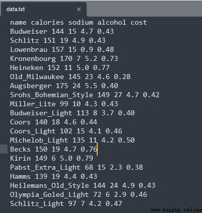
Code :
import pandas as pd
from sklearn.cluster import KMeans
from pandas.plotting import scatter_matrix
import matplotlib.pyplot as plt
import numpy as np
# Read data source
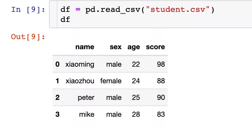
beer = pd.read_csv('E:/file/data.txt', sep=' ')
X = beer[["calories","sodium","alcohol","cost"]]
# Train two models , One 2 A cluster of , One 3 A cluster of
km = KMeans(n_clusters=3).fit(X)
km2 = KMeans(n_clusters=2).fit(X)
# Output model's label
print (" Model label:" , km.labels_)
# Add labels to the data source
beer['cluster'] = km.labels_
beer['cluster2'] = km2.labels_
print (" Add data after clustering labels :")
print(beer.sort_values('cluster'))
print (" Output clustering 2 The mean value of each eigenvalue :")
print(beer.groupby("cluster2").mean())
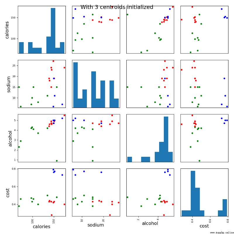
# pandas Draw a scatter plot
cluster_centers = km.cluster_centers_
cluster_centers_2 = km2.cluster_centers_
centers = beer.groupby("cluster").mean().reset_index()
plt.rcParams['font.size'] = 14
colors = np.array(['red', 'green', 'blue', 'yellow'])
scatter_matrix(beer[["calories","sodium","alcohol","cost"]],s=100, alpha=1, c=colors[beer["cluster"]], figsize=(10,10))
plt.suptitle("With 3 centroids initialized")
plt.show()
Test record :
 Model label: [1 1 1 1 1 1 1 1 0 0 1 0 1 1 1 2 1 1 2 0]
Add data after clustering labels :
name calories sodium ... cost cluster cluster2
9 Budweiser_Light 113 8 ... 0.40 0 1
11 Coors_Light 102 15 ... 0.46 0 1
8 Miller_Lite 99 10 ... 0.43 0 1
19 Schlitz_Light 97 7 ... 0.47 0 1
4 Heineken 152 11 ... 0.77 1 0
5 Old_Milwaukee 145 23 ... 0.28 1 0
6 Augsberger 175 24 ... 0.40 1 0
7 Srohs_Bohemian_Style 149 27 ... 0.42 1 0
2 Lowenbrau 157 15 ... 0.48 1 0
10 Coors 140 18 ... 0.44 1 0
1 Schlitz 151 19 ... 0.43 1 0
12 Michelob_Light 135 11 ... 0.50 1 0
13 Becks 150 19 ... 0.76 1 0
14 Kirin 149 6 ... 0.79 1 0
16 Hamms 139 19 ... 0.43 1 0
17 Heilemans_Old_Style 144 24 ... 0.43 1 0
3 Kronenbourg 170 7 ... 0.73 1 0
0 Budweiser 144 15 ... 0.43 1 0
18 Olympia_Goled_Light 72 6 ... 0.46 2 1
15 Pabst_Extra_Light 68 15 ... 0.38 2 1
[20 rows x 7 columns]
Output clustering 2 The mean value of each eigenvalue :
calories sodium alcohol cost cluster
cluster2
0 150.000000 17.000000 4.521429 0.520714 1.000000
1 91.833333 10.166667 3.583333 0.433333 0.666667

Code :
import pandas as pd
from sklearn.cluster import KMeans
from pandas.plotting import scatter_matrix
import matplotlib.pyplot as plt
import numpy as np
from sklearn.preprocessing import StandardScaler
# Read data source
beer = pd.read_csv('E:/file/data.txt', sep=' ')
X = beer[["calories","sodium","alcohol","cost"]]
# And process the data
scaler = StandardScaler()
X_scaled = scaler.fit_transform(X)
print (" Normalized data set :" )
print(X_scaled)
# Train two models , One 2 A cluster of , One 3 A cluster of
km = KMeans(n_clusters=3).fit(X_scaled)
km2 = KMeans(n_clusters=2).fit(X_scaled)
# Output model's label
print (" Model label:" , km.labels_)
# Add labels to the data source
beer['cluster'] = km.labels_
beer['cluster2'] = km2.labels_
print (" Add data after clustering labels :")
print(beer.sort_values('cluster'))
print (" Output clustering 2 The mean value of each eigenvalue :")
print(beer.groupby("cluster2").mean())
# pandas Draw a scatter plot
cluster_centers = km.cluster_centers_
cluster_centers_2 = km2.cluster_centers_
centers = beer.groupby("cluster").mean().reset_index()
plt.rcParams['font.size'] = 14
colors = np.array(['red', 'green', 'blue', 'yellow'])
scatter_matrix(beer[["calories","sodium","alcohol","cost"]],s=100, alpha=1, c=colors[beer["cluster"]], figsize=(10,10))
plt.suptitle("With 3 centroids initialized")
plt.show()
Test record :
 Normalized data set :
[[ 0.38791334 0.00779468 0.43380786 -0.45682969]
[ 0.6250656 0.63136906 0.62241997 -0.45682969]
[ 0.82833896 0.00779468 -3.14982226 -0.10269815]
[ 1.26876459 -1.23935408 0.90533814 1.66795955]
[ 0.65894449 -0.6157797 0.71672602 1.95126478]
[ 0.42179223 1.25494344 0.3395018 -1.5192243 ]
[ 1.43815906 1.41083704 1.1882563 -0.66930861]
[ 0.55730781 1.87851782 0.43380786 -0.52765599]
[-1.1366369 -0.7716733 0.05658363 -0.45682969]
[-0.66233238 -1.08346049 -0.5092527 -0.66930861]
[ 0.25239776 0.47547547 0.3395018 -0.38600338]
[-1.03500022 0.00779468 -0.13202848 -0.24435076]
[ 0.08300329 -0.6157797 -0.03772242 0.03895447]
[ 0.59118671 0.63136906 0.43380786 1.88043848]
[ 0.55730781 -1.39524768 0.71672602 2.0929174 ]
[-2.18688263 0.00779468 -1.82953748 -0.81096123]
[ 0.21851887 0.63136906 0.15088969 -0.45682969]
[ 0.38791334 1.41083704 0.62241997 -0.45682969]
[-2.05136705 -1.39524768 -1.26370115 -0.24435076]
[-1.20439469 -1.23935408 -0.03772242 -0.17352445]]
Model label: [0 0 1 2 2 0 0 0 1 1 0 1 1 2 2 1 0 0 1 1]
Add data after clustering labels :
name calories sodium ... cost cluster cluster2
0 Budweiser 144 15 ... 0.43 0 1
1 Schlitz 151 19 ... 0.43 0 1
17 Heilemans_Old_Style 144 24 ... 0.43 0 1
16 Hamms 139 19 ... 0.43 0 1
5 Old_Milwaukee 145 23 ... 0.28 0 1
6 Augsberger 175 24 ... 0.40 0 1
7 Srohs_Bohemian_Style 149 27 ... 0.42 0 1
10 Coors 140 18 ... 0.44 0 1
15 Pabst_Extra_Light 68 15 ... 0.38 1 0
12 Michelob_Light 135 11 ... 0.50 1 1
11 Coors_Light 102 15 ... 0.46 1 0
9 Budweiser_Light 113 8 ... 0.40 1 0
8 Miller_Lite 99 10 ... 0.43 1 0
2 Lowenbrau 157 15 ... 0.48 1 0
18 Olympia_Goled_Light 72 6 ... 0.46 1 0
19 Schlitz_Light 97 7 ... 0.47 1 0
13 Becks 150 19 ... 0.76 2 1
14 Kirin 149 6 ... 0.79 2 1
4 Heineken 152 11 ... 0.77 2 1
3 Kronenbourg 170 7 ... 0.73 2 1
[20 rows x 7 columns]
Output clustering 2 The mean value of each eigenvalue :
calories sodium alcohol cost cluster
cluster2
0 101.142857 10.857143 3.2 0.440000 1.000000
1 149.461538 17.153846 4.8 0.523846 0.692308
Calculate the sample i Average distance to other samples in the same cluster ai.ai The smaller it is , Explain the sample i The more it should be clustered into the cluster . take ai Called a sample i Within the cluster .
Calculate the sample i To some other cluster Cj The average distance of all samples bij, Called a sample i And clusters Cj The dissimilarity of . Defined as a sample i There is no similarity between clusters :bi =min{bi1, bi2, …, bik}
si near 1, Then the sample i Clustering is reasonable
si near -1, Then the sample i It should be classified into other clusters
if si Approximate 0, Then the sample i On the boundary of two clusters .
Code :
import pandas as pd
from sklearn.cluster import KMeans
from pandas.plotting import scatter_matrix
import matplotlib.pyplot as plt
import numpy as np
from sklearn.preprocessing import StandardScaler
from sklearn import metrics
# Read data source
beer = pd.read_csv('E:/file/data.txt', sep=' ')
X = beer[["calories","sodium","alcohol","cost"]]
# And process the data
scaler = StandardScaler()
X_scaled = scaler.fit_transform(X)
# Train two models , One is raw data , One is the normalized data
km = KMeans(n_clusters=3).fit(X)
km2 = KMeans(n_clusters=2).fit(X_scaled)
# Add labels to the data source
beer['cluster'] = km.labels_
beer['scaled_cluster'] = km2.labels_
score_scaled = metrics.silhouette_score(X,beer.scaled_cluster)
score = metrics.silhouette_score(X,beer.cluster)
print(" Output normalized score and raw data sample score :")
print(score_scaled, score)
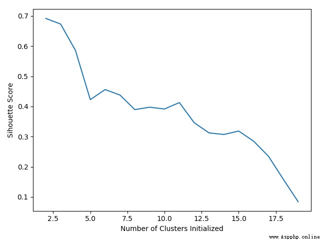
# View different K Score under value
scores = []
for k in range(2,20):
labels = KMeans(n_clusters=k).fit(X).labels_
score = metrics.silhouette_score(X, labels)
scores.append(score)
print(" View different K Value score :")
print(scores)
plt.plot(list(range(2,20)), scores)
plt.xlabel("Number of Clusters Initialized")
plt.ylabel("Sihouette Score")
plt.show()
Test record :
 Output normalized score and raw data sample score :
0.5562170983766765 0.6731775046455796
View different K Value score :
[0.6917656034079486, 0.6731775046455796, 0.5857040721127795, 0.422548733517202, 0.4559182167013377, 0.43776116697963124, 0.38946337473125997, 0.39746405172426014, 0.3915697409245163, 0.41282646329875183, 0.3459775237127248, 0.31221439248428434, 0.30707782144770296, 0.31834561839139497, 0.2849514001174898, 0.23498077333071996, 0.1588091017496281, 0.08423051380151177]
analysis :
After normalization , Actually, the effect is not as good as the original data set , It is estimated that the sample is too simple , In most cases, after normalization , The effect will be improved to a certain extent .