hello , Hello everyone .
Today, I'd like to introduce a practical case of machine learning that is very suitable for beginners .
This is a Housing forecast The case of , originate Kaggle Website , It is the first competition topic for many algorithm beginners .
This case has a complete process of solving machine learning problems , contain EDA、 Feature Engineering 、 model training 、 Model fusion, etc .
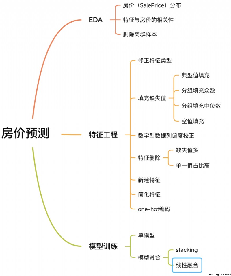
House price forecasting process
Now follow me , Let's learn about this case .
No wordy words , There's no extra code , Only popular explanations .
Exploratory data analysis (Exploratory Data Analysis, abbreviation EDA) The purpose of is to give us a full understanding of the data set . In this step , What we explore is as follows :

EDA Content
1.1 Input data set
train = pd.read_csv('./data/train.csv')
test = pd.read_csv('./data/test.csv')
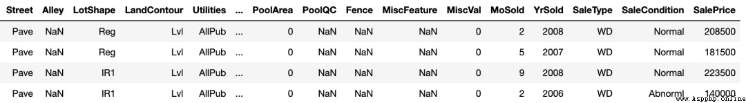
The training sample
train and test They are training set and test set , There were 1460 Samples ,80 Features .
SalePrice Column represents house price , It's what we want to predict .
1.2 House price distribution
Because our task is to predict house prices , Therefore, in the data set, the core concern is house prices (SalePrice) Value distribution of a column .
sns.distplot(train['SalePrice']);
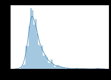
Value distribution of house price
As you can see from the diagram ,SalePrice The column peak is steep , And the peak value deviates to the left .
It can also be called directly skew() and kurt() Function calculation SalePrice Concrete skewness and kurtosis value .
about skewness and kurtosis Are relatively large , It is suggested that SalePrice List log() Smooth .
1.3 Characteristics related to house prices
To understand the SalePrice After the distribution of , We can calculate 80 Characteristics and SalePrice The relationship between .
Focus on and SalePrice The most relevant 10 Features .
#  Calculate correlation between columns
corrmat = train.corr()
#  take  top10
k = 10
cols = corrmat.nlargest(k, 'SalePrice')['SalePrice'].index
#  mapping
cm = np.corrcoef(train[cols].values.T)
sns.set(font_scale=1.25)
hm = sns.heatmap(cm, cbar=True, annot=True, square=True, fmt='.2f', annot_kws={'size': 10}, yticklabels=cols.values, xticklabels=cols.values)
plt.show()
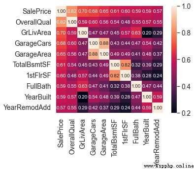
And SalePrice Highly correlated features
OverallQual( House materials and decoration )、GrLivArea( Aboveground living area )、GarageCars( Garage capacity ) and TotalBsmtSF( Basement area ) Follow SalePrice There's a strong correlation .
These features are done later Feature Engineering Will also focus on .
1.4 Eliminate outlier samples
Due to the small sample size of the data set , Outliers are not conducive to our later training model .
So you need to calculate each Numerical properties The outliers of , Eliminate the sample with the largest number of outliers .
#  Get numeric features
numeric_features = train.dtypes[train.dtypes != 'object'].index
#  Calculate outlier samples for each feature
for feature in numeric_features:
    outs = detect_outliers(train[feature], train['SalePrice'],top=5, plot=False)
    all_outliers.extend(outs)
#  Output the sample with the largest number of outliers
print(Counter(all_outliers).most_common())
#  Eliminate outlier samples
train = train.drop(train.index[outliers])
detect_outliers() It's a custom function , use sklearn Library LocalOutlierFactor Algorithm to calculate outliers .
Come here , EDA It's done. . Last , Merge training set and test set , Carry out the following feature Engineering .
y = train.SalePrice.reset_index(drop=True)
train_features = train.drop(['SalePrice'], axis=1)
test_features = test
features = pd.concat([train_features, test_features]).reset_index(drop=True)
features Combined the characteristics of training set and test set , It's the data we're going to deal with next .
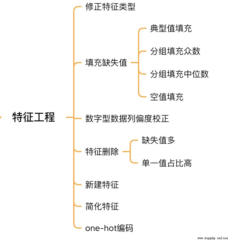
Feature Engineering
2.1 Correction feature type
MSSubClass( Type of house )、YrSold( Year of sale ) and MoSold( Sales month ) It is a category feature , It's just numbers , You need to turn them into text features .
features['MSSubClass'] = features['MSSubClass'].apply(str)
features['YrSold'] = features['YrSold'].astype(str)
features['MoSold'] = features['MoSold'].astype(str)
2.2 Fill feature missing value
There is no uniform standard for filling in missing values , You need to decide how to fill... According to different characteristics .
# Functional: Typical values are provided in the documentation Typ
features['Functional'] = features['Functional'].fillna('Typ') #Typ  It's a typical value
#  Group filling needs to be grouped according to similar characteristics , Take mode or median
# MSZoning( Housing area ) according to  MSSubClass( House ) Type group fill mode
features['MSZoning'] = features.groupby('MSSubClass')['MSZoning'].transform(lambda x: x.fillna(x.mode()[0]))
#LotFrontage( To receive examples ) Press Neighborhood Group fill median
features['LotFrontage'] = features.groupby('Neighborhood')['LotFrontage'].transform(lambda x: x.fillna(x.median()))
#  Numerical correlation of garage , Empty means none , Use 0 Fill in empty values .
for col in ('GarageYrBlt', 'GarageArea', 'GarageCars'):
    features[col] = features[col].fillna(0)
2.3 Skewness correction
Follow exploration SalePrice Columns are similar , Smooth the features with high skewness .
# skew() Method , Calculate the skewness of the feature (skewness).
skew_features = features[numeric_features].apply(lambda x: skew(x)).sort_values(ascending=False)
#  The skewness is greater than  0.15  Characteristics of
high_skew = skew_features[skew_features > 0.15]
skew_index = high_skew.index
#  Processing high skewness features , Turn it into a normal distribution , You can also use simple log Transformation
for i in skew_index:
    features[i] = boxcox1p(features[i], boxcox_normmax(features[i] + 1))
2.4 Feature deletion and addition
For almost all missing values , Or a single value accounts for a high proportion (99.94%) Features can be deleted directly .
features = features.drop(['Utilities', 'Street', 'PoolQC',], axis=1)
meanwhile , Multiple features can be fused , Generate new features .
Sometimes it is difficult for the model to learn the relationship between features , Manual feature fusion can reduce the difficulty of model learning , Improve the effect .
#  Merge the original construction date with the reconstruction date
features['YrBltAndRemod']=features['YearBuilt']+features['YearRemodAdd']
#  The basement area 、1 floor 、2 Floor area integration
features['TotalSF']=features['TotalBsmtSF'] + features['1stFlrSF'] + features['2ndFlrSF']
You can find , Our fusion is characterized by SalePrice Strongly correlated features .
Finally, simplify the features , For the characteristics of monotonic distribution ( Such as :100 Of the data 99 The value of one is 0.9, another 1 Yes 0.1), Conduct 01 Handle .
features['haspool'] = features['PoolArea'].apply(lambda x: 1 if x > 0 else 0)
features['has2ndfloor'] = features['2ndFlrSF'].apply(lambda x: 1 if x > 0 else 0)
2.6 Generate final training data
Here, the feature project is finished , We need to go from features Separate the training set and the test set again , Construct the final training data .
X = features.iloc[:len(y), :]
X_sub = features.iloc[len(y):, :]
X = np.array(X.copy())
y = np.array(y)
X_sub = np.array(X_sub.copy())
because SalePrice It is numerical and continuous , So we need to train one The regression model .
3.1 Single model the first Mod
First of all Ridge return (Ridge) For example , Construct a k Fold cross validation model .
from sklearn.linear_model import RidgeCV
from sklearn.pipeline import make_pipeline
from sklearn.model_selection import KFold
kfolds = KFold(n_splits=10, shuffle=True, random_state=42)
alphas_alt = [14.5, 14.6, 14.7, 14.8, 14.9, 15, 15.1, 15.2, 15.3, 15.4, 15.5]
ridge = make_pipeline(RobustScaler(), RidgeCV(alphas=alphas_alt, cv=kfolds))
Ridge return The model has a super parameter alpha, and RidgeCV The parameter name of is alphas, Represents entering a super parameter alpha Array . When fitting the model , From alpha Select a value that performs well in the array .
Because there is only one model now , Undetermined Ridge return Is it the best model . So we can find some models with high appearance rate and try more .
# lasso
lasso = make_pipeline(
    RobustScaler(),
    LassoCV(max_iter=1e7, alphas=alphas2, random_state=42, cv=kfolds))
#elastic net
elasticnet = make_pipeline(
    RobustScaler(),
    ElasticNetCV(max_iter=1e7, alphas=e_alphas, cv=kfolds, l1_ratio=e_l1ratio))
#svm
svr = make_pipeline(RobustScaler(), SVR(
    C=20,
    epsilon=0.008,
    gamma=0.0003,
))
#GradientBoosting( Expand to the first derivative )
gbr = GradientBoostingRegressor(...)
#lightgbm
lightgbm = LGBMRegressor(...)
#xgboost( Expand to the second derivative )
xgboost = XGBRegressor(...)
With multiple models , We can define another scoring function , Score the model .
# Model scoring function
def cv_rmse(model, X=X):
    rmse = np.sqrt(-cross_val_score(model, X, y, scoring="neg_mean_squared_error", cv=kfolds))
    return (rmse)
With Ridge return For example , Calculate the model score .
score = cv_rmse(ridge)
print("Ridge score: {:.4f} ({:.4f})\n".format(score.mean(), score.std()), datetime.now(), ) #0.1024
Run other models and find that the scores are almost the same .
At this time, we can choose any model , fitting , forecast , Submit training results . Or to Ridge return For example
#  Training models
ridge.fit(X, y)
#  Model to predict
submission.iloc[:,1] = np.floor(np.expm1(ridge.predict(X_sub)))
#  Output test results
submission = pd.read_csv("./data/sample_submission.csv")
submission.to_csv("submission_single.csv", index=False)
submission_single.csv Is the house price predicted by ridge regression , We can upload this result to Kaggle Check the score and ranking of the results on the website .
3.2 Model fusion -stacking
Sometimes in order to play the role of multiple models , We will integrate multiple models , This method is also called Integrated learning .
stacking It is a common Integrated learning Method . Simply speaking , It defines a metamodel , The output of other models is used as the input feature of the meta model , The output of the meta model will be the final prediction result .
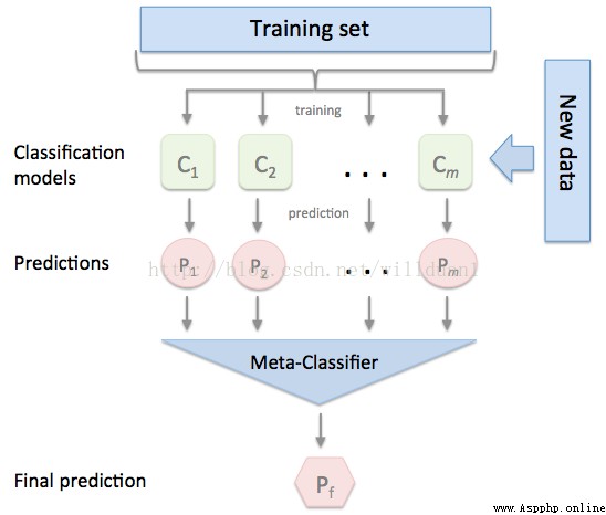
stacking
here , We use it mlextend In the library StackingCVRegressor modular , Do... On the model stacking.
stack_gen =
  StackingCVRegressor(
      regressors=(ridge, lasso, elasticnet, gbr, xgboost, lightgbm),
      meta_regressor=xgboost,
      use_features_in_secondary=True)
Training 、 The prediction process is the same as above , No more details here .
3.3 Model fusion - Linear fusion
The idea of multi model linear fusion is very simple , Assign a weight to each model ( Weight sum =1), The final prediction result takes the weighted average value of each model .
#  Train a single model
ridge_model_full_data = ridge.fit(X, y)
lasso_model_full_data = lasso.fit(X, y)
elastic_model_full_data = elasticnet.fit(X, y)
gbr_model_full_data = gbr.fit(X, y)
xgb_model_full_data = xgboost.fit(X, y)
lgb_model_full_data = lightgbm.fit(X, y)
svr_model_full_data = svr.fit(X, y)
models = [
    ridge_model_full_data, lasso_model_full_data, elastic_model_full_data,
    gbr_model_full_data, xgb_model_full_data, lgb_model_full_data,
    svr_model_full_data, stack_gen_model
]
#  Assign model weights
public_coefs = [0.1, 0.1, 0.1, 0.1, 0.15, 0.1, 0.1, 0.25]
#  Linear fusion , Take the weighted average
def linear_blend_models_predict(data_x,models,coefs, bias):
    tmp=[model.predict(data_x) for model in models]
    tmp = [c*d for c,d in zip(coefs,tmp)]
    pres=np.array(tmp).swapaxes(0,1)
    pres=np.sum(pres,axis=1)
    return pres
Come here , Housing forecast We have finished explaining the case of , You can run it yourself , Look at the model effects trained in different ways .
Reviewing the whole case will find that , We have spent a lot of time on data preprocessing and Feature Engineering , Although the principle of machine learning problem model is difficult to learn , But in the actual process, feature engineering often takes the most thought .
Full source code for official account :Python Source code Can get