Pandas statistical analysis (date data processing, time series, downsampling, upsampling, excel multi table consolidation, stock market data analysis, solving Chinese garbled code)
編輯:Python
This blog post is from 《Python Data analysis goes from beginner to proficient 》_ Edited by tomorrow Technology
4.8 Date data processing
4.8.1 DataFrame Date data conversion
On a daily basis , A very troublesome thing is that the format of dates can be expressed in many ways , We see the same 2020 year 2 month 14 Japan , There can be many formats , Pictured 4.57 Shown . that , We need to unify these formats before we can carry out the follow-up work .Pandas Provides to_datetime() Methods can help us solve this problem .
to_datetime() Method can be used to batch process date data conversion , It is very practical and convenient for processing big data , It can convert date data into various formats you need . for example , take 2/14/20 and 14-2-2020 Convert to date format 2020-02-14.to_datetime() The syntax of the method is as follows :
arg: character string 、 Date time 、 Array of strings
errors: The value is ignore、raise or coerce, The details are as follows , The default value is ignore, That is, ignore the error . – ignore: Invalid parsing will return the original value – raise: Invalid parsing will throw an exception – coerce: Invalid resolution will be set to NaT, That is, data that cannot be converted to date will be converted to NaT
dayfirst: The first is the day , Boolean type , The default value is False. for example 02/09/2020, If the value is True, Then the first of the parsing date is day , namely 2020-09-02; If the value is False, The resolution date is the same as the original date , namely 2020-02-09
yearfirst: The first is year , Boolean type , The default value is False. for example 14-Feb-20, If the value is True, Then the first of the parsing date is year , namely 2014-02-20; If the value is False, The resolution date is the same as the original date , namely 2020-02-14
utc: Boolean type , The default value is None. return utc Coordinate world time
box: Boolean value , The default value is True, If the value is True, Then return to DatatimeIndex; If the value is False, Then return to ndarray.
format: Format the display time . character string , The default value is None
exact: Boolean value , The default value is True, If True, The format must match exactly ; If False, Allows the format to match anywhere in the target string
unit: The default value is None, Unit of parameter (D、s、ms、us、ns) A unit of time
infer_datetime_format: The default value is False. If there is no format , Then try to infer the format from the first date time string .
origin: The default value is unix. Define reference date . The value will be resolved to a unit number
cache: The default value is False. If the value is True, Then unique 、 The cache of the conversion date applies the time conversion of the date . Parsing duplicate date string , Especially for strings with time zone offset , There may be significant acceleration . Only if at least 50 Cache is used only when there are values . The existence of an out of range value will make the cache unusable , And may slow down parsing .
Return value : Date time
Convert various date strings to the specified date format
take 2020 year 2 month 14 Various formats of the day are converted to date format , The program code is as follows :
import pandas as pd
df=pd.DataFrame({
' Original date ':['14-Feb-20', '02/14/2020', '2020.02.14', '2020/02/14','20200214']})
df[' Date after conversion ']=pd.to_datetime(df[' Original date '])
print(df)
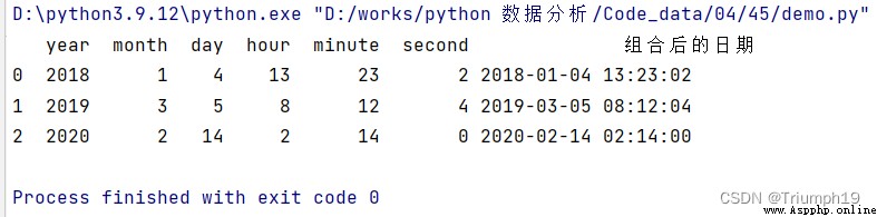
It can also be realized from DataFrame Multiple columns in the object , Like a year 、 month 、 The columns of the day are combined into one column of the day . Date abbreviations commonly used in key value . Combination requirements :
import pandas as pd
df = pd.DataFrame({
'year': [2018, 2019,2020],
'month': [1, 3,2],
'day': [4, 5,14],
'hour':[13,8,2],
'minute':[23,12,14],
'second':[2,4,0]})
df[' Date after combination ']=pd.to_datetime(df)
print(df)
4.8.2 dt Use of objects
dt The object is Series Object to get the date attribute , Through it, you can get the year in the date 、 month 、 Japan 、 Weeks 、 Seasons, etc , You can also judge whether the date is at the end of the year . The grammar is as follows :
Series.dt()
Return value : Return the same index series as the original series . If Series Date value is not included , It causes a mistake .
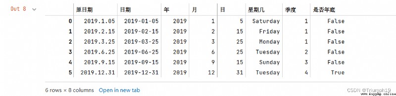
dt The object provides year、month、day、dayofweek、dayofyear、is_leap_year、quarter、weekday_name Other properties and methods . for example ,year Can get " year "、quarter You can directly get the quarter of each date ,weekday_name You can directly get the day of the week corresponding to each date .
Gets the year in the date 、 month 、 Japan 、 Number of weeks, etc
import pandas as pd
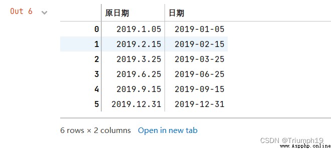
df=pd.DataFrame({
' Original date ':['2019.1.05', '2019.2.15', '2019.3.25','2019.6.25','2019.9.15','2019.12.31']})
df[' date ']=pd.to_datetime(df[' Original date '])
df
df[' year '],df[' month '],df[' Japan ']=df[' date '].dt.year,df[' date '].dt.month,df[' date '].dt.day
df[' What day ']=df[' date '].dt.day_name()
df[' quarter ']=df[' date '].dt.quarter
df[' Whether the end of the year ']=df[' date '].dt.is_year_end
df
4.8.3 Get the data of the date range
The method to obtain the data of the date range is directly in DataFrame Object to enter a date or date range , but The date must be set as the index , Examples are as follows :
obtain 2018 Years of data
df1['2018']
obtain 2017-2018 Years of data
df1['2017':'2018']
Get a month (2018 year 7 month ) The data of
df1['2018-07']
Get the specific day (2018 year 5 month 6 Japan ) The data of
df1['2018-05-06':'2018-05-06']
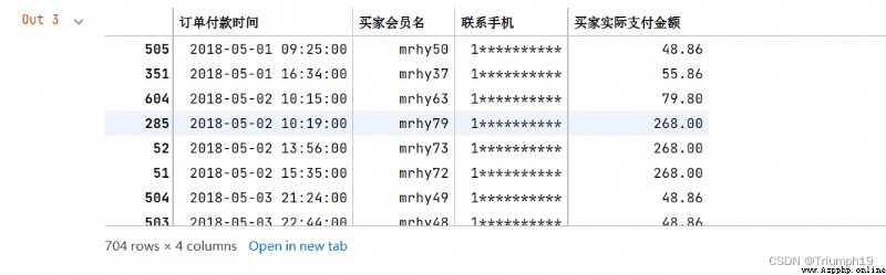
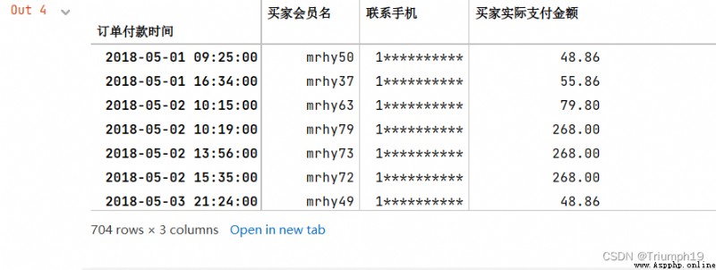
Get the order data of the specified date range
obtain 2018 year 5 month 11 solstice 6 month 10 Order of day , The results are shown in the following figure
import pandas as pd
df = pd.read_excel('mingribooks.xls')
df1=df[[' Order payment time ',' Buyer member name ',' Contact your cell phone ',' The actual amount paid by the buyer ']]
df1=df1.sort_values(by=[' Order payment time '])
df1
df1 = df1.set_index(' Order payment time ') # Set the date to index
df1
# Get the data of a certain interval
df2=df1['2018-05-11':'2018-06-10']
df2
4.8.4 Statistics and display data by different periods
1. Statistics by period
Statistics by period are mainly through DataFrame Object's resample() Method combined with data calculation function .resample() The method is mainly applied to time series frequency conversion and resampling , It can get the year from the date 、 month 、 Japan 、 week 、 Seasons, etc , Combined with the data calculation function, we can achieve year 、 month 、 Japan 、 Statistics of different periods such as week or quarter . An example is shown below . Index must be of date type .
(1) Annual statistics , The code is as follows :
df1=df1.resample('AS').sum()
(2) Quarterly statistics , The code is as follows :
df2.resample('Q').sum()
(3) According to monthly statistics , The code is as follows :
df1.resample('M').sum()
(4) Statistics by week , The code is as follows :
df1.resample('W').sum()
(5) Statistics by day , The code is as follows :
df1.resample('D').sum()
2. Display data by period
DataFrame Object's to_period() Method can convert a timestamp to a period , So as to display data by date , The premise is that the date must be set to index . The grammar is as follows :
DataFrame.to_period(freq=None,axis=0,copy=True)
freq: character string , Frequency of periodic index , The default value is None
axis: Row column index ,axis=0 Indicates the row index ,axis=1 Indicates column index . The default value is 0, That is, the row index .
copy: Whether to copy data , The default value is True, If the value is False, Data is not copied .
Return value : Time series with periodic index
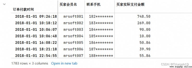
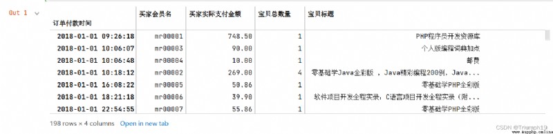
Get different periods from dates
Get different periods from dates , The main codes are as follows :
import pandas as pd
aa =r'TB2018.xls'
df = pd.DataFrame(pd.read_excel(aa))
df1=df[[' Order payment time ',' Buyer member name ',' Contact your cell phone ',' The actual amount paid by the buyer ']]
df1 = df1.set_index(' Order payment time ') # take date Set to index
df1
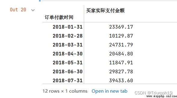
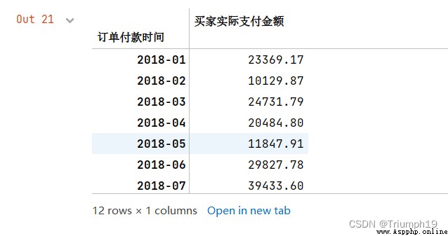
Monthly statistics
# Monthly statistics
#“MS” The first day of each month is the start date ,“M” It's the last day of every month
df1.resample('M').sum()
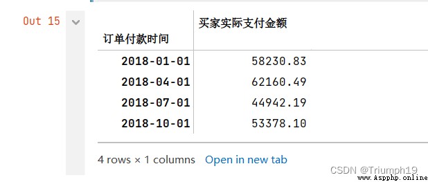
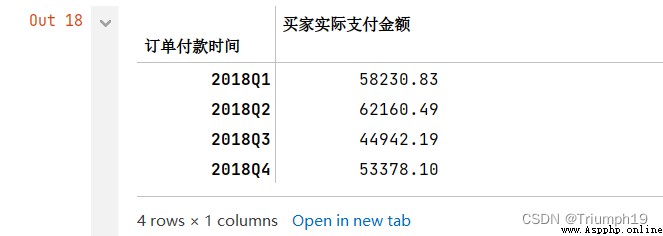
Quarterly statistics
# Quarterly statistics
#“QS” The first day of each quarter is the start date ,“Q” It's the last day of each quarter
df1.resample('QS').sum()
Annual statistics
# Annual statistics
#“AS” Is the first day of each year as the start date ,“A” It's the last day of every year
df1.resample('AS').sum()
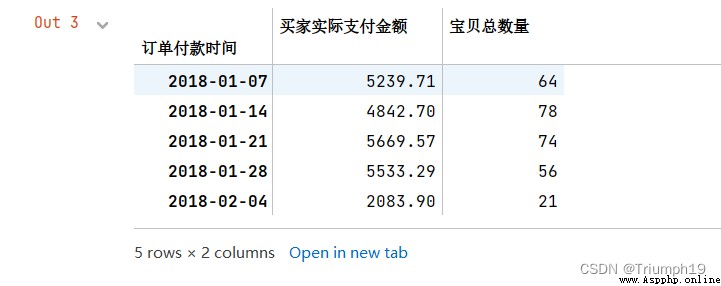
Statistics by year and display data
# Statistics by year and display data
#“AS” Is the first day of each year as the start date ,“A” It's the last day of every year
df1.resample('AS').sum().to_period('A')
Statistics and display data by quarter
# Statistics and display data by quarter
df1.resample('Q').sum().to_period('Q')
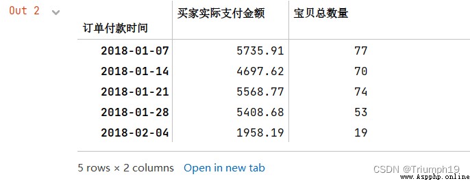
Statistics by month and display data
# Monthly statistics
#“MS” The first day of each month is the start date ,“M” It's the last day of every month
df1.resample('M').sum().to_period('M')
Count and display data by week
df1.resample('w').sum().to_period('W').head()
4.9 The time series
4.9.1 Resampling (Resample() Method )
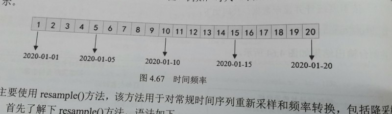
Through the previous study , We learned how to generate time indexes of different frequencies , By hour 、 By day 、 By week 、 Monthly, etc , If you want to convert data with different frequencies , What should I do ? stay Pandas The adjustment of the frequency of time series in is called resampling , That is, the process of converting time series from one frequency to another . for example , One frequency per day is converted to every 5 One frequency per day , Pictured 4.67 Shown .
Resampling mainly uses resample() Method , This method is used for resampling and frequency conversion of conventional time series , Including down sampling and up sampling . First of all, understand resample() Method , The grammar is as follows :
rule: character string , The offset represents the target string or object transformation
how: Function name or array function used to generate aggregate values . for example mean、ohlc and np.max etc. , The default value is mean, Other commonly used values are first、last、median、max and min.
axis: integer , Represents a row or column ,axis=0 The column ,axis=1 Said line . The default value is 0, That is, the column
fill_method: Fill method used for L sampling ,fill() Method ( Fill with the previous value ) or bfill() Method ( Fill in with the post value ), The default value is None
closed: When downsampling , Opening and closing of time interval , Same as the concept of interval in mathematics , Its value is right or left,right Indicates left opening and right closing ,left Indicates left closed right open , The default value is right Left open right closed
label: When downsampling , How to label aggregate values . for example ,10:30-10:35 Will be marked as 10:30 still 10:35, The default value is None
convention: When resampling , The convention used to convert low frequencies to high frequencies , Its value is start or end, The default value is start
kind: It's time to get together (period) Or timestamp (timestamp), Default index type aggregated to time series , The default value is None.
loffset: The time correction value of the aggregate tag , The default value is None. for example ,-1s or second(-1) Used to set the aggregation label early 1 second
limit: Fill forward or backward , The maximum number of periods allowed to be filled , The default value is None
base: integer , The default value is 0. For uniform subdivision 1 The frequency of the day , Aggregate interval " origin ". for example , about 5min frequency ,base The scope can be 0~4
on: character string , Optional parameters , The default value is None. Yes DataFrame Object uses columns instead of indexes for resampling . The column must be similar to the date time
level: character string , Optional parameters , The default value is None. For multiple indexes , Resampled level or level number , The level must be similar to the date time
Return value : Resample the object
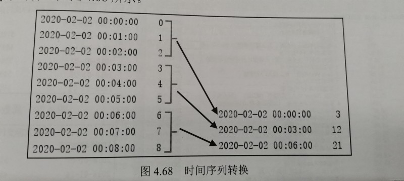
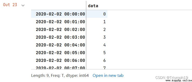
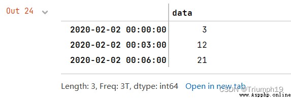
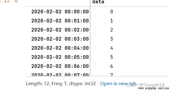
A one minute time series translates into 3 Minute time series
First create an include 9 A one minute time series , And then use resample() Method to 3 Minute time series , And calculate the sum of the index , Pictured 4.68 Shown .
The program code is as follows :
import pandas as pd
index = pd.date_range('02/02/2020', periods=9, freq='T')
series = pd.Series(range(9), index=index)
series
series.resample('3T').sum()
4.9.2 Downsampling processing
Downsampling is the transition of the period from high frequency to low frequency . for example , take 5min Stock trading data is converted into daily trading , The sales data counted by day is converted into weekly statistics .
Data downsampling involves data aggregation . for example , Day data becomes week data , Then you have to be right 1 Zhou 7 Data of days are aggregated , The way of aggregation mainly includes summation 、 Find the mean, etc .
Statistics of sales data by week
import pandas as pd
df=pd.read_excel('time.xls')
df1 = df.set_index(' Order payment time ') # Set up “ Order payment time ” Index
df1
df1.resample('W').sum().head()
#%%
df1.resample('W',closed='left').sum()
4.9.3 L sampling processing
The upsampling is the transition from low frequency to high frequency . When converting data from low frequency to high frequency , There is no need for aggregation , Resample it to daily frequency , Missing values will be introduced by default .
for example , It turned out to be weekly statistics , Now it turns to statistics by day . Liter sampling involves data filling , According to the filling method , The filled data is also different . Here are three filling methods . – No fill . Null value uses NaN Instead of , Use asfreq() Method . – Fill with the previous value . Fill in the empty values with the preceding values , Use ffill() Methods or pad() Method . For the convenience of memory ,ffill() Method can use its first letter "f" Instead of , representative forward, Forward means . – Fill in with the post value , Use bfill() Method , You can use letters "b" Instead of , representative back, Backward means .
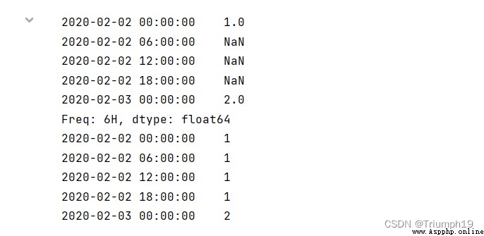
Every time 6 Make statistics every hour
Now create a time series , The start date is 2020-02-02, A total of two days , The corresponding values of each day are 1 and 2, Each... Is processed by liter sampling 6 Make statistics every hour , Null values are filled in different ways , The program code is as follows :
import pandas as pd
import numpy as np
rng = pd.date_range('20200202', periods=2)
s1 = pd.Series(np.arange(1,3), index=rng)
s1
In Finance , I often see the opening (open)、 The close (close)、 Highest price (high) And the lowest price (low) data , And in the Pandas The resampled data in can also achieve such results , By calling ohlc() Function to get the result of data summary , That is, the starting value (open)、 End value (close)、 Maximum value (high) And the lowest value (low).ohlc() The syntax of the function is as follows :
resample.ohlc()
ohlc() The function returns DataFrame object , Of each group of data open( open )、high( high )、low( low ) and close( Turn off ) value .
Statistical data open、high、low and close value .
Each group below 5 Minute time series , adopt ohlc() Function to get the start value of each group of time in the time series 、 Maximum value 、 Minimum and end values , The program code is as follows :
import pandas as pd
import numpy as np
rng = pd.date_range('2/2/2020',periods=12,freq='T')
s1 = pd.Series(np.arange(12),index=rng)
s1
s1.resample('5min').ohlc()
4.9.5 Move window data calculation (rolling() function )
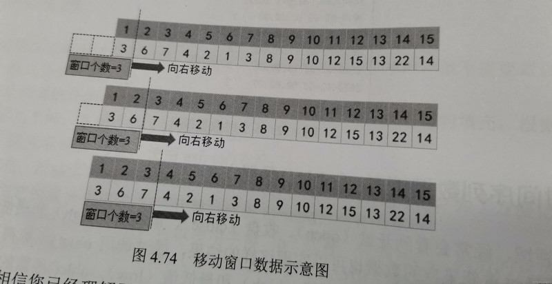
Through resampling, you can get any low-frequency data you want , But these data are also the data of common time points , Then there is such a problem : The data at the time point fluctuates greatly , The data at a certain point cannot well express its own characteristics , So there was " Move the window " The concept of , In short , In order to improve the reliability of data , Expand the value of a point to a range of this point , Use intervals to judge , This section is the window .
Here's an example , chart 4.74 The schematic diagram of moving window data is displayed , The time series represents 1 Number to 15 Daily sales data on the th , Next, let's say 3 A window for , Move the window from left to right , According to the statistics 3 The average value of days is taken as the value of this point , Such as 3 The sales volume of No. is 1 Number 、2 Number and 3 The average value of number .
I believe you have understood the mobile window through the above schematic diagram , stay Pandas Through rolling() Function to realize the calculation of moving window data , The grammar is as follows :
window: The size of the time window , There are two forms , namely int or offset. If you use int, Then the numerical value represents the number of observations for calculating the statistics , That is, the forward data ; If you use offset, Represents the size of the time window .
min_periods: The minimum number of observations per window , Windows less than this result in NA. Values can be int, The default value is None.offset Under the circumstances , The default value is 1
center: Set the label of the window to play . Boolean type , The default value is False, be at the right
win_type: The type of window . All kinds of functions that intercept windows . String type , The default value is None
on: Optional parameters . about DataFrame object , Is to specify the column to calculate the moving window , The value is the column name
axis: integer ,axis=0 The column ,axis=1 Said line . The default value is 0, That is to calculate the column
closed: Define the opening and closing of an interval , Support int Type of window . about offset The default type is left open right closed . It can be specified according to the situation left.
Return value : A subclass of a window or moving window generated for a specific operation
Create Taobao daily sales data
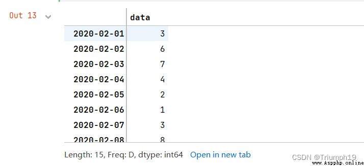
First, create a set of Taobao daily sales data , The program code is as follows :
import pandas as pd
index=pd.date_range('20200201','20200215')
data=[3,6,7,4,2,1,3,8,9,10,12,15,13,22,14]
s1_data=pd.Series(data,index=index)
s1_data
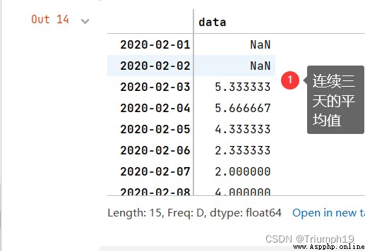
Use rolling() Function calculation 3 The average of days
Use rolling() Function calculation 2020-02-01 to 2020-02-15 in 3 The average of days , The number of windows is 3, The code is as follows :
s1_data.rolling(3).mean()
Run the program , look down rolling() How is the function calculated ? When the window starts moving , First time 2020-02-01 And the second time point 2020-02-02 The value of is empty , This is because the number of windows is 3, There is empty data in front of them , So the mean is empty ; And to the third time point 2020-02-03 when , The data in front of it is 2020-02-01 to 2020-02-03, therefore 3 The average of days is 5033333; And so on .
Use the data of the day to represent the window data
In calculating the first time point 2020-02-01 Window data , Although the data is not enough window length 3, But at least the data of the day , Can we use the data of the day to represent the window data ? The answer is yes , By setting min_periods Parameters can be , It represents the minimum number of observations in the window , The window length less than this value is displayed as empty , There is a value when it is equal to or greater than , The main codes are as follows :
s1_data.rolling(3,min_periods=1).mean()
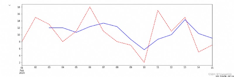
import numpy as np
import pandas as pd
index=pd.date_range('20200201','20200215')
data=[3,6,7,4,2,1,3,8,9,10,12,15,13,22,14]
np.random.seed(2)
data=np.random.randint(20,size=len(index))
ser_data=pd.Series(data,index=index)
plt.figure(figsize=(15, 5))
ser_data.plot(style='r--')
ser_data.rolling(3).mean().plot(style='b')
4.10 Comprehensive application
Case study 1:Excel Merging multiple tables
In daily work , Almost every day, we have a lot of data to process , The desktop is always covered with Excel surface , It looks very messy , In fact, we can have the same category Excel Merge tables together , In this way, data will not be lost , And it can also analyze data very effectively . Use concat() Method to specify all Excel Table merge , The program code is as follows :
import pandas as pd
import glob
filearray=[]
filelocation=glob.glob(r'./aa/*.xlsx') # Specify all... In the directory Excel file # Traverse the specified directory for filename in filelocation: filearray.append(filename) print(filename) res=pd.read_excel(filearray[0]) # Read the first Excel file # Sequential read Excel File and merge for i in range(1,len(filearray)): A=pd.read_excel(filearray[i]) res=pd.concat([res,A],ignore_index=True,sort=False) # Ignore the index , See pandas In statistical analysis print(res.index) # write in Excel file , And save writer = pd.ExcelWriter('all.xlsx') res.to_excel(writer,'sheet1') writer.save()
4.10.2 Case list 2: Stock market data analysis
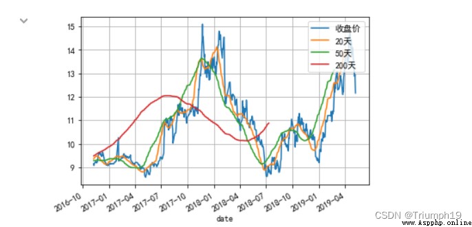
Stock data includes opening price 、 Closing price 、 The lowest price 、 Trading volume and other indicators . among , The closing price is the standard of the day's market , It is also the basis for the opening price of the next trading day , It can predict the future stock market , So when investors analyze the market , Generally, the closing price is used as the valuation basis .
Use rolling() Function to calculate a stock 20 God 、50 Days and 200 The average closing price of the day and generate a trend chart ( Also known as K Line graph ), The program code is as follows :
import pandas as pd
import numpy as np
import matplotlib.pyplot as plt
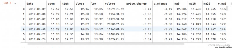
aa =r'000001.xlsx'
df = pd.DataFrame(pd.read_excel(aa))
df['date'] = pd.to_datetime(df['date']) # Convert data type to date type
df
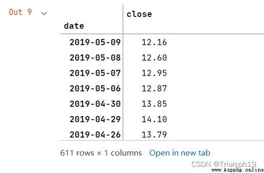
df = df.set_index('date') # take date Set to index
df=df[['close']] # Extract closing price data
df
df['20 God '] = np.round(df['close'].rolling(window = 20, center = False).mean(), 2)
df['50 God '] = np.round(df['close'].rolling(window = 50, center = False).mean(), 2)
df['200 God '] = np.round(df['close'].rolling(window = 200, center = False).mean(), 2)
plt.rcParams['font.sans-serif']=['SimHei'] # Solve the Chinese garbled code
df.plot(secondary_y = [" Closing price ", "20","50","200"], grid = True)
plt.legend((' Closing price ','20 God ', '50 God ', '200 God '), loc='upper right')