This article describes how to Matplotlib Use in LaTeX Formulas and symbols 、Python How to generate LaTeX The mathematical formula .

1、Matplotlib Use in LaTeX Formulas and symbols

Some configurations

• Install two software , Link given .

• https://mirrors.cqu.edu.cn/CTAN/systems/windows/protext/protext-3.2-033020.zip

• https://github.com/ArtifexSoftware/ghostpdl-downloads/releases/download/gs9531/gs9531w64.exe

• Add to environment variable

Put the following two sentences in the environment variable .C:\Users\xx\AppData\Local\Programs\MiKTeX 2.9\miktex\bin\x64;C:\Program Files\gs\gs9.53.1\bin;

• matplotlib.rcParams modify

import numpy as np
import matplotlib as mpl
import matplotlib.pyplot as plt
plt.style.use('fivethirtyeight')
mpl.rcParams['text.usetex'] = True# The default is false, This is set to TRUE

Matplotlib Use in Latex Characters and formulas

mpl.rcParams['lines.linewidth'] = 1
fig, ax = plt.subplots(dpi=120)
N = 500
delta = 0.6
X = np.linspace(-1, 1, N)
ax.plot(X, (1 - np.tanh(4 * X / delta)) / 2,    
        X, (1.4 + np.tanh(4 * X / delta)) / 4, "C2", 
        X, X < 0, "k--")                        
 
ax.set_xlabel(r'No.1: $\alpha > \beta)
# The subscript , Superscript ^, Subscript
ax.set_ylabel(r'No.2: $\alpha_i > \beta^i,rotation=45)
# # Add up 、 The cumulative
ax.legend((r'No.3: $\displaystyle\sum_{i=0}^\infty x_i, r'No.4: $\displaystyle\prod_{i=0}^\infty x_i),
          shadow=True, loc=(0.01, 0.52), handlelength=1.5, )
# fraction   
ax.set_title(r'No.4: $\frac{3}{4})
# binomial
ax.text(0.3,1.1,r'No.5: $\frac{5 - \frac{1}{x}}{4})
# Square root
ax.text(0.8,1.1,r'No.6: $\sqrt[3]{x})
# Change the font
## Roman、Italic、Typewriter、CALLIGRAPHY etc.
ax.text(-0.8,1.1,r'No.7: $\mathit{Italic})
ax.text(-0.8,1.0,r'$\mathsf{fonts})
# tone
ax.text(-1.2,1.1,r'No.8: $\breve a)
# Select a range
ax.text(-1.4,0.8,r'No.9: $\widetilde{xyz})
# the arrow
ax.annotate("", xy=(-delta / 2., 0.1), xytext=(delta / 2., 0.1),
            arrowprops=dict(arrow, connection))
#   Other TeX symbols
ax.set_xticks([-1, 0, 1])
ax.set_xticklabels([r"No.10: $\delta$", r"$\pm$", r"$\$"], color="r", size=15)
ax.set_yticks([0, 0.5, 1])
ax.set_yticklabels([r"No.10: $\AA$", r"$\Downarrow$", "$\\odot$"], color="r", size=15)
ax.text(1.02, 0.5, r"$\phi$",fontsize=20, rotation=90,
        horizontalalignment="left", verticalalignment="center",
        clip_on=False, transform=ax.transAxes)
#  integral 、 Differential formula
eq1 = (r"\begin{eqnarray*}"
       r"\frac{\partial \phi}{\partial t} + U|\nabla \phi| &=& 0 "
       r"\end{eqnarray*}")
ax.text(1, 0.9, eq1,horizontalalignment="right", verticalalignment="top")
eq2 = (r"\begin{eqnarray*}"
       r"\mathcal{F} &=& \int f\left( \phi, c \right) dV, \\ "
       r"\frac{ \partial \phi } { \partial t } &=& -M_{ \phi } "
       r"\frac{ \delta \mathcal{F} } { \delta \phi }"
       r"\end{eqnarray*}")
ax.text(0.18, 0.18, eq2)
ax.text(-1, .30, r"gamma: $\gamma$", color="r")
ax.text(-1, .18, r"Omega: $\Omega$", color="b")
plt.show()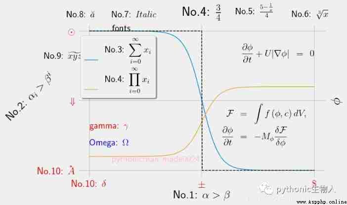

2、latexify Generate LaTeX The mathematical formula

import math
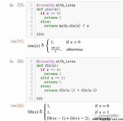
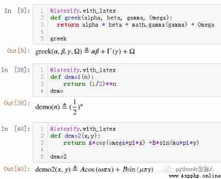
import latexify
@latexify.with_latex# call latexify The decorator
def solve(a, b, c):
  return (-b + math.sqrt(b**2 - 4*a*c)) / (2*a)
solve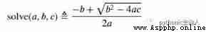

3、handcalcs Generate LaTeX The mathematical formula

• An integral formula , With the help of scipy Of quad

import handcalcs.render
from scipy.integrate import quad# With the help of scipy.quad Realize integral 

%%render
a = 2
b = 6
n=100
z = quad(f,a,b)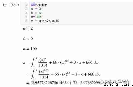

• A mixed formula , With the help of math modular ,

from math import sqrt,cos,sin,tan,asin
import handcalcs.render

%%render
#symbolic
f = a-c**2 / b + sqrt(cos(sin(b- 2 / c))) + tan(a/b) - asin(a/c) #Comment part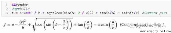

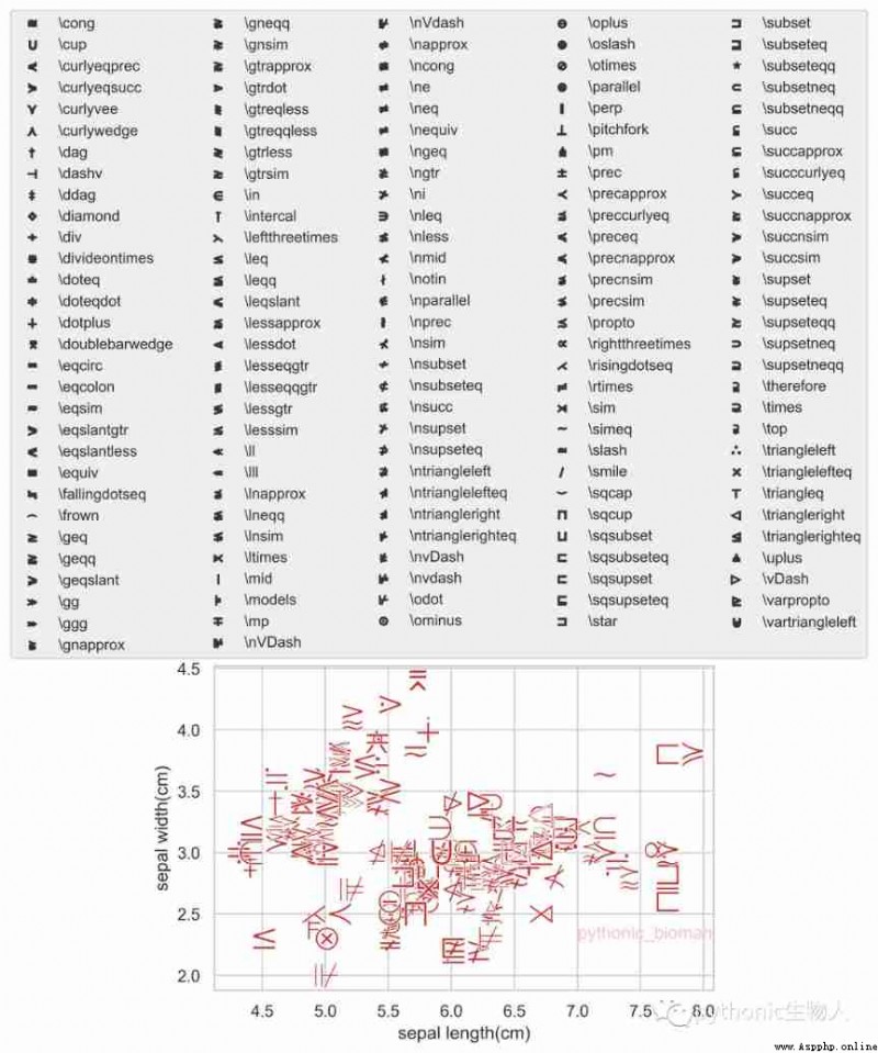
4、Latex symbols Comparison table

symbols Climb from the website ：https://matplotlib.org/tutorials/text/mathtext.html、 Make a quick look-up table .

plt.figure(dpi=400)
fig = sns.scatterplot(x='sepal length(cm)',y='sepal width(cm)',data=pd_iris,
            style=geek[:150],# Add different variables according to different marker Show
            markers=[r"$"+geek[i]+"$" for i in range(150)],# Customize marker shape
            **dict(s=320),
            color='#01a2d9'
                      
           )
fig.legend(ncol=5,
           fontsize=10,
           loc=8,
           bbox_to_anchor=(0.45, 1), 
           facecolor='#eaeaea',          
          )
sns.set(,font_scale=1)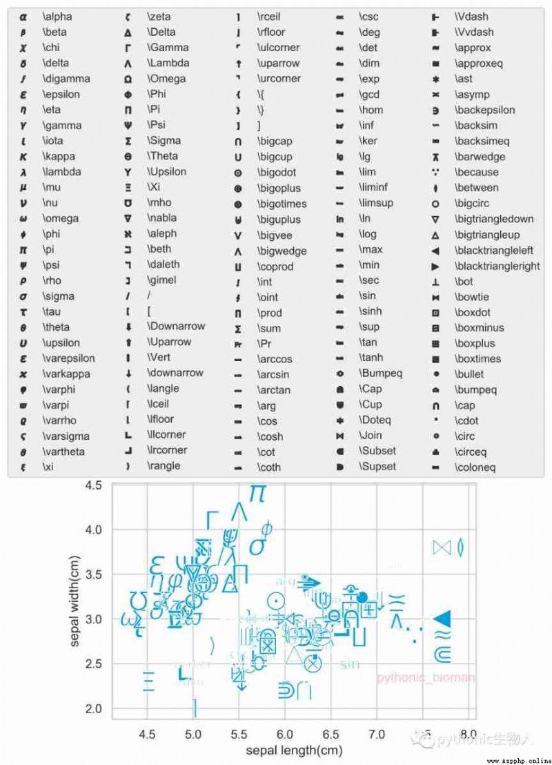

Reference material

https://matplotlib.org/tutorials/text/usetex.html
https://github.com/connorferster/handcalcs
https://github.com/google/latexify_py

-END-

 Past highlights
It is suitable for beginners to download the route and materials of artificial intelligence ( Image & Text + video ) Introduction to machine learning series download Chinese University Courses 《 machine learning 》（ Huang haiguang keynote speaker ） Print materials such as machine learning and in-depth learning notes 《 Statistical learning method 》 Code reproduction album
AI Basic download machine learning communication qq Group 955171419, Please scan the code to join wechat group ：