Separate the two different types of texture areas on the left and right in the following figure , The output result of the method is a binary image of the same size as the image , On the left for 0, On the right is 1, Or vice versa , Grey border lines are not considered in the design method , Self removal .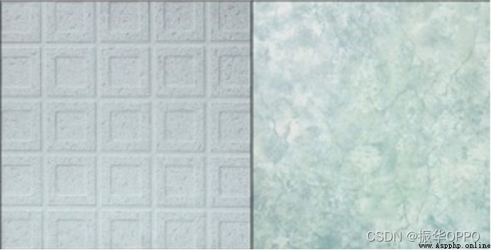
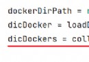
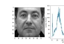
import matplotlib.image as mpimgimport matplotlib.pyplot as pltimport numpy as npfrom cv2 import cv2from sklearn.multiclass import OneVsRestClassifierfrom sklearn.svm import SVRfrom skimage import feature as skftfrom PIL import Image,ImageDraw,ImageFontclass Texture(): #n_point Select the number of pixels around the central pixel #radius Radius of the selected area def __init__(self): self.radius = 1 self.n_point = self.radius * 8 # Load grayscale image def loadPicture(self): train_index = 0 test_index = 0 train_data = np.zeros((10, 171, 171)) test_data = np.zeros((8, 171, 171)) train_label = np.zeros(10) test_label = np.zeros(8) for i in np.arange(2): image = mpimg.imread('dataset1/'+str(i)+'.tiff') data = np.zeros((513, 513)) data[0:image.shape[0], 0:image.shape[1]] = image index = 0 # Picture division 9 block ,5 Block training 4 Block prediction for row in np.arange(3): for col in np.arange(3): if index < 5: train_data[train_index, :, :] = data[171*row:171*(row+1),171*col:171*(col+1)] train_label[train_index] = i train_index += 1 else: test_data[test_index, :, :] = data[171*row:171*(row+1),171*col:171*(col+1)] test_label[test_index] = i test_index += 1 index += 1 return train_data, test_data, train_label, test_label # Texture detection def texture_detect(self): train_data, test_data, train_label, test_label = self.loadPicture() n_point = self.n_point radius = self.radius train_hist = np.zeros((10, 256)) test_hist = np.zeros((8, 256)) #LBP feature extraction for i in np.arange(10): # Use LBP Method to extract the texture features of the image . lbp=skft.local_binary_pattern(train_data[i], n_point, radius, 'default') # Histogram of statistical image max_bins = int(lbp.max() + 1) # hist size:256 train_hist[i], _ = np.histogram(lbp, normed=True, bins=max_bins, range=(0, max_bins)) for i in np.arange(8): lbp = skft.local_binary_pattern(test_data[i], n_point, radius, 'default') max_bins = int(lbp.max() + 1) # hist size:256 test_hist[i], _ = np.histogram(lbp, normed=True, bins=max_bins, range=(0, max_bins)) return train_hist, test_hist # Training classifier SVM Support vector machine classification def classifer(self): train_data, test_data, train_label, test_label = self.loadPicture() train_hist, test_hist = self.texture_detect() # structure SVM Support vector machine svr_rbf = SVR(kernel='rbf', C=1e3, gamma=0.1) model= OneVsRestClassifier(svr_rbf, -1) model.fit(train_hist, train_label) image=cv2.imread('dataset1/image.png',cv2.IMREAD_GRAYSCALE) image=cv2.resize(image,(588,294)) img_ku=skft.local_binary_pattern(image,8,1,'default') thresh=cv2.adaptiveThreshold(image,255,cv2.ADAPTIVE_THRESH_GAUSSIAN_C,cv2.THRESH_BINARY,11,2) # Recognize and classify images img_data=np.zeros((1,98,98)) data=np.zeros((294,588)) data[0:image.shape[0],0:image.shape[1]]=image img = Image.open('texture.png') draw = ImageDraw.Draw(img) # Set font and size myfont = ImageFont.truetype('C:/windows/fonts/Arial.ttf', size=180) # Set font color fillcolor = "#008B8B" # For reading pictures size, That is, width and height width, height = img.size # Divide the image into nine blocks by rows and columns for row in np.arange(3): for col in np.arange(6): img_data[0,:,:]=data[98*row:98*(row+1),98*col:98*(col+1)] lbp= skft.local_binary_pattern(img_data[0], 8, 1, 'default') max_bins=int(lbp.max()+1) img_hist, _ = np.histogram(lbp, normed=True, bins=max_bins, range=(0, max_bins)) predict=model.predict(img_hist.reshape(1,-1)) if(predict==0): draw.text((width/6, height/6), '0', font=myfont, fill=fillcolor) data[98*row:98*(row+1),98*col:98*(col+1)]=0 else: draw.text((2*width /3, height/6), '1', font=myfont, fill=fillcolor) data[98*row:98*(row+1),98*col:98*(col+1)]=255 plt.subplot(211) plt.imshow(img_ku,'gray') #plt.subplot(312) #plt.imshow(thresh,'gray') plt.subplot(212) plt.imshow(img) plt.show()if __name__ == '__main__': test = Texture() # Calculate the classification accuracy accuracy = test.classifer() #print('Final Accuracy = '+str(accuracy)+'%') The picture above shows the result LBP Image after operator feature extraction , The following figure uses SVM The result of texture classification , The same as the predicted upper left texture is marked as 0, The same as the above figure on the right is marked as 1.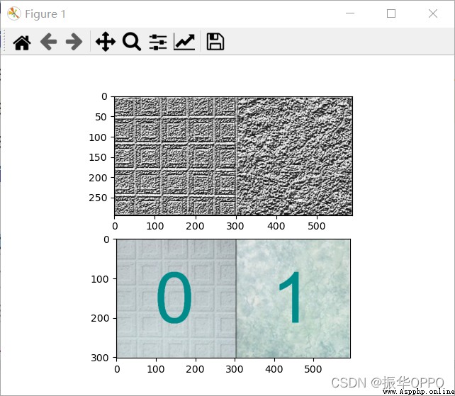
stay Linux In the major distributions of ,Ubuntu And its derivatives have always enjoyed the reputation of being user-friendly .Ubuntu It's an open source operating system , Its system and software can be found on the official website (http://cn.ubuntu.com) As a free download , Detailed installation instructions are provided .