 Predict whether hotel reviews are positive or negative :
1. The room is great , It's very close to the main road , Very convenient , Pretty good . Praise 0.9954
2. The room is a little dirty , The toilet is still leaking , The air conditioner fails to cool the air , I'll never come again . Bad review 0.99
3. The floor is not very clean , The TV has no signal , But the air conditioner is OK , Anyway, it's OK . Praise 0.56
pip3 install nltk -i
https://pypi.tuna.tsinghua.edu.cn/simple/
pip3 install jieba -i
https://pypi.tuna.tsinghua.edu.cn/simple/
import nltk.tokenize as tk
# Split the sample into sentences sent_list: List of sentences
sent_list = tk.sent_tokenize(text)
# Split the sample according to the list word_list: List of words
word_list = tk.word_tokenize(text)
# Split the sample into words punctTokenizer: Participator object
punctTokenizer = tk.WordPunctTokenizer()
word_list = punctTokenizer.tokenize(text)
doc = "Are you curious about tokenization? Let's see how it works! We need to analyze a couple of sentences with punctuations to see it in action."
# Separate sentences
sents = tk.sent_tokenize(doc)
for i in range(len(sents)):
print(i+1, ':', sents[i])
""" 1 : Are you curious about tokenization? 2 : Let's see how it works! 3 : We need to analyze a couple of sentences with punctuations to see it in action. """
# Word segmentation
words = tk.word_tokenize(doc)
for i in range(len(words)):
print(i+1, ':', words[i])
""" 1 : Are 2 : you 3 : curious 4 : about 5 : tokenization 6 : ? 7 : Let 8 : 's 9 : see 10 : how 11 : it 12 : works 13 : ! 14 : We 15 : need 16 : to 17 : analyze 18 : a 19 : couple 20 : of 21 : sentences 22 : with 23 : punctuations 24 : to 25 : see 26 : it 27 : in 28 : action 29 : . """
tokenizer = tk.WordPunctTokenizer()
words = tokenizer.tokenize(doc)
for i in range(len(words)):
print(i+1, ':', words[i])
""" 1 : Are 2 : you 3 : curious 4 : about 5 : tokenization 6 : ? 7 : Let 8 : ' 9 : s 10 : see 11 : how 12 : it 13 : works 14 : ! 15 : We 16 : need 17 : to 18 : analyze 19 : a 20 : couple 21 : of 22 : sentences 23 : with 24 : punctuations 25 : to 26 : see 27 : it 28 : in 29 : action 30 : . """
This hotel is very bad. The toilet in this hotel smells bed. The environment of this hotel is very good.
This hotel is very bad.
The toilet in this hotel smells bed.
The environment of this hotel is very good.
import sklearn.feature_extraction.text as ft
# Build bag model objects
cv = ft.CountVectorizer()
# Training models , Take all possible words in the sentence as feature names , Each sentence is a sample , The number of times a word appears in a sentence is the eigenvalue
bow = cv.fit_transform(sentences).toarray()
print(bow)
# Get all feature names
words = cv.get_features_names()
import sklearn.feature_extraction.text as ft
sents = ['This hotel is very bad.',
'The toilet in this hotel smells bad.',
'The environment of this hotel is very good.']
cv = ft.CountVectorizer()
bow = cv.fit_transform(sents)
print(bow)
print(bow.toarray())
print(cv.get_feature_names())
""" (0, 9) 1 (0, 3) 1 (0, 5) 1 (0, 11) 1 (0, 0) 1 (1, 9) 1 (1, 3) 1 (1, 0) 1 (1, 8) 1 (1, 10) 1 (1, 4) 1 (1, 7) 1 (2, 9) 1 (2, 3) 1 (2, 5) 1 (2, 11) 1 (2, 8) 1 (2, 1) 1 (2, 6) 1 (2, 2) 1 [[1 0 0 1 0 1 0 0 0 1 0 1] [1 0 0 1 1 0 0 1 1 1 1 0] [0 1 1 1 0 1 1 0 1 1 0 1]] ['bad', 'environment', 'good', 'hotel', 'in', 'is', 'of', 'smells', 'the', 'this', 'toilet', 'very'] """
 This hotel is great , Decoration stick , Breakfast bar , The environment is great . 1
This hotel sucks , Rotten rotten rotten , It really sucks . 0
The hotel is well decorated , Poor service . ?
writing files frequency rate : D F = contain Yes some individual single word Of writing files sample Ben Count total writing files sample Ben Count ( And sample Ben language The righteous Tribute offer degree back phase Turn off ) Document frequency : DF = \frac{ Sample number of documents containing a word }{ Total number of document samples }( It is inversely related to the semantic contribution of the sample ) writing files frequency rate :DF= total writing files sample Ben Count contain Yes some individual single word Of writing files sample Ben Count ( And sample Ben language The righteous Tribute offer degree back phase Turn off )
The inverse writing files frequency rate : I D F = l o g ( total sample Ben Count 1 + contain Yes some individual single word Of sample Ben Count ) ( And sample Ben language The righteous Tribute offer degree just phase Turn off ) Reverse document frequency : IDF = log\left(\frac{ The total number of samples }{1+ The number of samples containing a word }\right)( It is positively correlated with the semantic contribution of the sample ) The inverse writing files frequency rate :IDF=log(1+ contain Yes some individual single word Of sample Ben Count total sample Ben Count )( And sample Ben language The righteous Tribute offer degree just phase Turn off )
# Build bag model objects
cv = ft.CountVectorizer()
# Training models , Take all possible words in the sentence as feature names , Each sentence is a sample , The number of times a word appears in a sentence is the eigenvalue
bow = cv.fit_transform(sentences).toarray()
# obtain TF-IDF Model trainer
tt = ft.TfidfTransformer()
tfidf = tt.fit_transform(bow).toarray()
tt = ft.TfidfTransformer()
tfidf = tt.fit_transform(bow).toarray()
print(np.round(tfidf, 3))
print(cv.get_feature_names())
""" [[0.488 0. 0. 0.379 0. 0.488 0. 0. 0. 0.379 0. 0.488] [0.345 0. 0. 0.268 0.454 0. 0. 0.454 0.345 0.268 0.454 0. ] [0. 0.429 0.429 0.253 0. 0.326 0.429 0. 0.326 0.253 0. 0.326]] ['bad', 'environment', 'good', 'hotel', 'in', 'is', 'of', 'smells', 'the', 'this', 'toilet', 'very'] """
import numpy as np
import pandas as pd
import sklearn.datasets as sd
import sklearn.model_selection as ms
import sklearn.linear_model as lm
import sklearn.metrics as sm
# Load data set
data = sd.load_files('20news', encoding='latin1')
len(data.data) # 2968 Samples
""" 2968 """
import sklearn.feature_extraction.text as ft
# Organize input and output sets TFIDF Turn each email into an eigenvector
cv = ft.CountVectorizer()
bow = cv.fit_transform(data.data)
tt = ft.TfidfTransformer()
tfidf = tt.fit_transform(bow)
# tfidf.shape # (2968,40605)
# Split test set and training set
train_x, test_x, train_y, test_y = ms.train_test_split(tfidf, data.target, test_size=0.1, random_state=7)
# Cross validation
model = lm.LogisticRegression()
scores = ms.cross_val_score(model, tfidf, data.target, cv=5, scoring='f1_weighted')
# f1 score
print(scores.mean()) # 0.9597980963781605
# Training models
model.fit(train_x, train_y)
# test model , Evaluation model
pred_test_y = model.predict(test_x)
print(sm.classification_report(test_y, pred_test_y))
""" 0.9597980963781605 precision recall f1-score support 0 0.81 0.96 0.88 57 1 0.97 0.89 0.93 65 2 1.00 0.95 0.97 61 3 1.00 1.00 1.00 54 4 1.00 0.95 0.97 60 accuracy 0.95 297 macro avg 0.96 0.95 0.95 297 weighted avg 0.96 0.95 0.95 297 """
# Arrange a group of test samples for model test
test_data = ["In the last game, the spectator was accidentally hit by a baseball injury and has been hospitalized.",
"Recently, Lao Wang is studying asymmetric encryption algorithms.",
"The two-wheeled car is pretty good on the highway."]
# Convert the sample into... According to the training method tfidf matrix , Can be handed over to the model for prediction
bow = cv.transform(test_data)
test_data = tt.transform(bow)
pred_test_y = model.predict(test_data)
print(pred_test_y)
print(data.target_names)
""" [2 0 1] ['misc.forsale', 'rec.motorcycles', 'rec.sport.baseball', 'sci.crypt', 'sci.space'] """
data.target_names
""" ['misc.forsale', 'rec.motorcycles', 'rec.sport.baseball', 'sci.crypt', 'sci.space'] """
Probability reflects the probability of random events . A random event is a random event under the same conditions , Events that may or may not occur . for example :
(1) Flip a coin , Maybe face up , Maybe the opposite side is up , This is a random event . just / The possibility that the opposite side is up is called probability ;
(2) Dice , The number of points thrown is a random event . The probability of the occurrence of each point is called probability ;
(3) A batch of goods contains good products 、 Defective product , Take one at random , Good smoke / Defective products are random events . After a lot of trial and error , The defective rate is getting closer and closer to a constant , Then the constant is probability .
We can record random events as A or B, be P(A), P(B) Indicates an event A or B Probability .
It refers to the probability that multiple conditions are included and all conditions are true at the same time , Write it down as P ( A , B ) P ( A , B ) P(A,B) , or P ( A B ) P(AB) P(AB), or P ( A ⋂ B ) P(A \bigcap B) P(A⋂B)
Known events B Under the condition of occurrence , Take retail as an example A The probability of occurrence is called conditional probability , Write it down as : P ( A ∣ B ) P(A|B) P(A∣B)
p( It's raining | overcast )
event A It doesn't affect events B Happen , Call the two events independent , Write it down as :
P ( A B ) = P ( A ) P ( B ) P(AB)=P(A)P(B) P(AB)=P(A)P(B)
because A and B Do not affect each other , Then there are :
P ( A ∣ B ) = P ( A ) P(A|B) = P(A) P(A∣B)=P(A)
It can be understood as , Given or not given B Under the condition of ,A The probability is the same .
A priori probability is also the probability obtained from previous experience and analysis , for example : Without any information , Guess the last name of the stranger opposite , The probability of surnamed Li is the greatest ( Because the surname Li accounts for the highest proportion in the country ), This is a priori probability .
A posteriori probability refers to the correction probability when certain conditions or information are received , for example : I know that the person opposite is from “ Niujia village ” Under the circumstances , The probability of guessing his surname is the greatest , But the surname Yang is not ruled out 、 Lee, wait , This is a posteriori probability .
It hasn't happened yet , Find out the possibility of this happening , It's a priori probability ( It can be understood as seeking results ). It's happened , The reason for this event is the possibility caused by a certain factor , It's a posterior probability ( From the fruit to the cause ). There is an inseparable relationship between a priori probability and a posteriori probability , The calculation of posterior probability should be based on prior probability .
Bayes gave the reason to Thomas, an English mathematician . Bayes ( Thomas Bayes) Put forward , Used to describe the relationship between two conditional probabilities , The theorem is described as :
P ( A ∣ B ) = P ( A ) P ( B ∣ A ) P ( B ) P(A|B) = \frac{P(A)P(B|A)}{P(B)} P(A∣B)=P(B)P(A)P(B∣A)
among , P ( A ) P(A) P(A) and P ( B ) P(B) P(B) yes A Events and B The probability of an event happening . P ( A ∣ B ) P(A|B) P(A∣B) It's called conditional probability , Express B Under the condition of the event ,A The probability of an event happening . Derivation process :
P ( A , B ) = P ( B ) P ( A ∣ B ) P ( B , A ) = P ( A ) P ( B ∣ A ) P(A,B) =P(B)P(A|B)\\ P(B,A) =P(A)P(B|A) P(A,B)=P(B)P(A∣B)P(B,A)=P(A)P(B∣A)
among P ( A , B ) P(A,B) P(A,B) It's called joint probability , Refers to an event B Probability of occurrence , Times the event A In the event B The probability of occurrence under the condition of occurrence . because P ( A , B ) = P ( B , A ) P(A,B)=P(B,A) P(A,B)=P(B,A), So there is :
P ( B ) P ( A ∣ B ) = P ( A ) P ( B ∣ A ) P(B)P(A|B)=P(A)P(B|A) P(B)P(A∣B)=P(A)P(B∣A)
Divide both sides at the same time P(B), Then we get the expression of Bayesian Theorem . among , P ( A ) P(A) P(A) It's a priori probability , P ( A ∣ B ) P(A|B) P(A∣B) Is known B After occurrence A Conditional probability of , Also known as a posteriori probability .
Suppose a school 60% Of boys and 40% The girl of , The number of girls wearing trousers is equal to the number of girls wearing skirts , All the boys wear pants , A man looks at it in the distance at random , Look at a student in pants , May I ask the probability that this student is a girl :
p( Woman ) = 0.4
p( The trousers | Woman ) = 0.5
p( The trousers ) = 0.8
P( Woman | The trousers ) = 0.4 * 0.5 / 0.8 = 0.25
P ( A ∣ B ) = P ( A ) P ( B ∣ A ) P ( B ) P(A|B) = \frac{P(A)P(B|A)}{P(B)} P(A∣B)=P(B)P(A)P(B∣A)
import sklearn.naive_bayes as nb
# Create Gaussian naive Bayesian classifier object
model = nb.GaussianNB()
model = nb.MultinomialNB()
model.fit(x, y)
result = model.predict(samples)
GaussianNB It is more suitable for training samples that obey Gaussian distribution
MultinomialNB It is more suitable for training samples subject to multinomial distribution
stay sklearn in , Three naive Bayesian classifiers are provided , Namely :
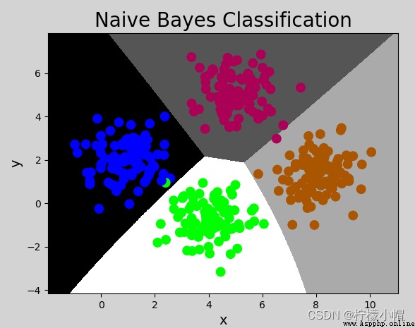
In the example , The value of the sample is continuous , And normal distribution , So using GaussianNB Model . The code is as follows :
# Naive Bayesian classification example
import numpy as np
import sklearn.naive_bayes as nb
import matplotlib.pyplot as mp
# Input , Output
x, y = [], []
# Read data file
with open("../data/multiple1.txt", "r") as f:
for line in f.readlines():
data = [float(substr) for substr in line.split(",")]
x.append(data[:-1]) # The input samples : Take from the first column to the penultimate column
y.append(data[-1]) # The output samples : Take the last column
x = np.array(x)
y = np.array(y, dtype=int)
# Create Gaussian naive Bayesian classifier object
model = nb.GaussianNB()
model.fit(x, y) # Training
# Calculate the display range
left = x[:, 0].min() - 1
right = x[:, 0].max() + 1
buttom = x[:, 1].min() - 1
top = x[:, 1].max() + 1
grid_x, grid_y = np.meshgrid(np.arange(left, right, 0.01),
np.arange(buttom, top, 0.01))
mesh_x = np.column_stack((grid_x.ravel(), grid_y.ravel()))
mesh_z = model.predict(mesh_x)
mesh_z = mesh_z.reshape(grid_x.shape)
mp.figure('Naive Bayes Classification', facecolor='lightgray')
mp.title('Naive Bayes Classification', fontsize=20)
mp.xlabel('x', fontsize=14)
mp.ylabel('y', fontsize=14)
mp.tick_params(labelsize=10)
mp.pcolormesh(grid_x, grid_y, mesh_z, cmap='gray')
mp.scatter(x[:, 0], x[:, 1], c=y, cmap='brg', s=80)
mp.show()
import numpy as np
import pandas as pd
import sklearn.datasets as sd
import sklearn.model_selection as ms
import sklearn.linear_model as lm
import sklearn.metrics as sm
# Load data set
data = sd.load_files('20news', encoding='latin1')
import sklearn.feature_extraction.text as ft
# Organize input and output sets TFIDF Turn each email into an eigenvector
cv = ft.CountVectorizer()
bow = cv.fit_transform(data.data)
tt = ft.TfidfTransformer()
tfidf = tt.fit_transform(bow)
# tfidf.shape # (2968,40605)
# Split test set and training set
train_x, test_x, train_y, test_y = ms.train_test_split(tfidf, data.target, test_size=0.1, random_state=7)
# Cross validation
# Using naive Bayes
import sklearn.naive_bayes as nb
model = nb.MultinomialNB()
scores = ms.cross_val_score(model, tfidf, data.target, cv=5, scoring='f1_weighted')
# f1 score
print(scores.mean())
# Training models
model.fit(train_x, train_y)
# test model , Evaluation model
pred_test_y = model.predict(test_x)
print(sm.classification_report(test_y, pred_test_y))
""" 0.9458384770112502 precision recall f1-score support 0 1.00 0.84 0.91 57 1 0.94 0.94 0.94 65 2 0.95 0.97 0.96 61 3 0.90 1.00 0.95 54 4 0.97 1.00 0.98 60 accuracy 0.95 297 macro avg 0.95 0.95 0.95 297 weighted avg 0.95 0.95 0.95 297 """
# Arrange a group of test samples for model test
test_data = ["In the last game, the spectator was accidentally hit by a baseball injury and has been hospitalized.",
"Recently, Lao Wang is studying asymmetric encryption algorithms.",
"The two-wheeled car is pretty good on the highway.",
"Next year, China will explore Mars."]
# Convert the sample into... According to the training method tfidf matrix , Can be handed over to the model for prediction
bow = cv.transform(test_data)
test_data = tt.transform(bow)
pred_test_y = model.predict(test_data)
print(pred_test_y)
print(data.target_names)
""" [2 3 1 4] ['misc.forsale', 'rec.motorcycles', 'rec.sport.baseball', 'sci.crypt', 'sci.space'] """
① advantage
② shortcoming