[Python artificial intelligence] Python full stack system (17)
編輯:Python
Artificial intelligence
The fifth chapter Vehicle rating classification and cart Classification tree
One 、 Decision tree classification
1. The core principle of the algorithm
The core idea of decision tree : Similar inputs produce similar outputs .
2. The key problem of decision tree
So many features , Which feature is used to divide the row sub table first ?
3. CART Classification tree
CART Classification tree algorithm bisects each feature , The Gini coefficient is used to express the purity of the data set when finding the split point , The smaller the Gini coefficient , The lower the impurity , The better the result of data set partition .
CART The process of classifying a tree into molecular tables :
For each feature , Calculate the optimal segmentation value based on Gini coefficient . In the data set of each segment value of each calculated feature D D D In the Gini coefficient of , Select the feature with the smallest Gini coefficient A And the corresponding split value a. According to this optimal feature and optimal segmentation value , Divide the data set into two parts D 1 D_1 D1 and D 2 D_2 D2, At the same time, establish the left and right nodes of the current node , The data set of the left node D D D by D 1 D_1 D1, The data set of the right node D D D by D 2 D_2 D2. Recursively call this procedure on the child nodes of the left and right nodes , Generate decision tree .
and CART The classification tree also determines the order in which the sub table divides the selected features based on the Gini coefficient .
4. The gini coefficient
For samples D, The number is |D|, hypothesis K Categories , The first k The number of categories is C k C_k Ck, Then the sample D Gini coefficient expression : G i n i ( D ) = 1 − ∑ i = 1 K ( ∣ C k ∣ ∣ D ∣ ) 2 Gini(D) = 1 - \sum_{i=1}^K \left(\frac{|C_k|}{|D|}\right)^2 Gini(D)=1−i=1∑K(∣D∣∣Ck∣)2
Yes 100 Samples ( D 1 D_1 D1) contain A And B Two categories , The quantities are 40 And 60,Gini( D 1 D_1 D1) = ? 1 − ( ( ∣ 40 ∣ ∣ 100 ∣ ) 2 + ( ∣ 60 ∣ ∣ 100 ∣ ) 2 ) = 1 − ( 0.16 + 0.36 ) = 0.48 1 - \left( \left(\frac{|40|}{|100|}\right)^2 + \left( \frac{|60|}{|100|}\right)^2 \right) = 1 - (0.16 + 0.36) = 0.48 1−((∣100∣∣40∣)2+(∣100∣∣60∣)2)=1−(0.16+0.36)=0.48
Yes 100 Samples ( D 2 D_2 D2) contain A And B Two categories , The quantities are 10 And 90,Gini( D 2 D_2 D2) = ? 1 − ( ( ∣ 10 ∣ ∣ 100 ∣ ) 2 + ( ∣ 90 ∣ ∣ 100 ∣ ) 2 ) = 1 − ( 0.01 + 0.81 ) = 0.18 1 - \left( \left( \frac{|10|}{|100|}\right)^2 + \left( \frac{|90|}{|100|}\right)^2 \right) = 1 - (0.01 + 0.81) = 0.18 1−((∣100∣∣10∣)2+(∣100∣∣90∣)2)=1−(0.01+0.81)=0.18
For samples D, The number is |D|, According to the characteristics of A A value of a, hold D Divide into D 1 D_1 D1 and D 2 D_2 D2, be In character A Under the condition of , sample D Gini coefficient expression by : G i n i ( D , A ) = ∣ D 1 ∣ ∣ D ∣ G i n i ( D 1 ) + ∣ D 2 ∣ ∣ D ∣ G i n i ( D 2 ) Gini(D,A) = \frac{|D_1|}{|D|} Gini(D_1) + \frac{|D_2|}{|D|} Gini(D_2) Gini(D,A)=∣D∣∣D1∣Gini(D1)+∣D∣∣D2∣Gini(D2)
5. The generation process of decision tree
Algorithm input training set D, Threshold of Gini coefficient , Sample number threshold . Output decision tree T.
For the current node, the data set is D, If the number of samples is less than the threshold , Then return to decision tree , The current node stops recursion .
Calculate the sample set D Gini coefficient of , If the Gini coefficient is less than the threshold , Then return to the decision tree subtree , The current node stops recursion .
Calculate each eigenvalue pair data set of the existing features of the current node D Gini coefficient of .
In the calculation of each feature of each characteristic value pair data set D In the Gini coefficient of , Select the feature with the smallest Gini coefficient A And the corresponding eigenvalues a. According to this optimal characteristic and optimal eigenvalue , Divide the data set into two parts D 1 D_1 D1 and D 2 D_2 D2, At the same time, establish the left and right nodes of the current node , The data set of the left node D by D 1 D_1 D1, The data set of the right node D by D 2 D_2 D2.
Recursive calls to the left and right child nodes 1-4 Step , Generate decision tree .
The prediction process : When making predictions for the generated decision tree , If the sample in the test set A It's on a leaf node , There are multiple training samples in the node . For A The category prediction uses the category with the highest probability in this leaf node .
6. Decision tree classification implementation
Decision tree classifier model correlation API:
import sklearn.tree as st
# Decision tree classifier
model = st.DecisionTreeClassifier(
max_depth=6, min_samples_split=3, random_state=7)
model.fit(train_x, train_y)
7. Iris case
import sklearn.tree as st
model = st.DecisionTreeClassifier(max_depth=4, min_samples_split=3)
model.fit(train_x, train_y)
# assessment Model accuracy
pred_test_y = model.predict(test_x)
print((pred_test_y==test_y).sum() / test_y.size)
print(test_y.values)
""" 0.8666666666666667 [2 0 0 1 0 2 2 2 1 1 2 1 1 0 0] """
8. Set model classification implementation
Common classifiers provided by the set model
import sklearn.ensemble as se
model = se.RandomForestClassifier(...) # Random forest classifier
model = se.AdaBoostClassifier(...) # AdaBoost classifier
model = se.GridientBoostingClassifier(...) # GBDT classifier
Two 、 Predict car rating
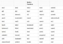
car.txt In the sample file, the common characteristic information of cars and the classification of cars are counted , These data are used to train the model to predict the car grade based on the decision tree classification algorithm .
Car price Maintenance costs Number of doors Number of passengers trunk Security Car grade
Analysis of implementation ideas :
Load data .
Feature analysis and feature engineering .
Data preprocessing ( Tag code ).
Training models .
Model test .
import numpy as np
import pandas as pd
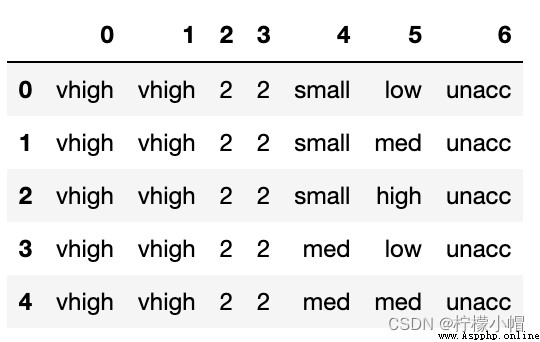
data = pd.read_csv('car.txt', header=None) # I don't want to use the first line as the header
data.head()
data[0].value_counts() # Car price sharing 4 class , By category, each category has 432 Samples
""" vhigh 432 low 432 med 432 high 432 Name: 0, dtype: int64 """
determine : It's about classification , Or the question of return ? answer : classification
Which classification model to choose : Logical regression 、 Decision tree 、RF、GBDT、AdaBoost? answer :RF( Of course, you can also try other models )
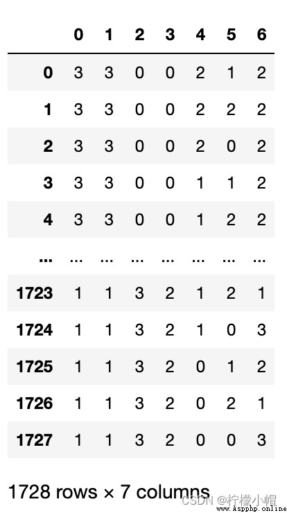
# Complete label coding preprocessing for the current group of data
import sklearn.preprocessing as sp
# Traverse each column of data
train_data = pd.DataFrame([])
encoders = {
}
for col_ind, col_val in data.items():
encoder = sp.LabelEncoder()
train_data[col_ind] = encoder.fit_transform(col_val)
encoders[col_ind] = encoder
train_data
# Organize input and output sets
x, y = train_data.iloc[:, :-1], train_data[6]
x.shape, y.shape
""" ((1728, 6), (1728,)) """
# Create a classification model
model = se.RandomForestClassifier(max_depth=6, n_estimators=400, random_state=7)
# do 5 Secondary cross validation , Verify that this model is available
scores = ms.cross_val_score(model, x, y, cv=5, scoring='f1_weighted')
# If the score is OK , A more serious training model
print(scores.mean())
""" 0.7537201013972693 """
# Model to evaluate ( First, use training samples to evaluate the model )
model.fit(x, y)
pred_y = model.predict(x)
print(sm.classification_report(y, pred_y))
print(sm.confusion_matrix(y,pred_y)) # hold 1 Total attribution of categories 0 Category
""" precision recall f1-score support 0 0.77 0.82 0.79 384 1 0.00 0.00 0.00 69 2 0.95 0.99 0.97 1210 3 1.00 0.77 0.87 65 accuracy 0.91 1728 macro avg 0.68 0.65 0.66 1728 weighted avg 0.87 0.91 0.89 1728 [[ 315 0 69 0] [ 69 0 0 0] [ 11 0 1199 0] [ 15 0 0 50]] """
data = [
['high', 'med', '5more', '4', 'big', 'low', 'unacc'],
['high', 'high', '4', '4', 'med', 'med', 'acc'],
['low', 'low', '2', '4', 'small', 'high', 'good'],
['low', 'med', '3', '4', 'med', 'high', 'vgood']
]
test_data = pd.DataFrame(data)
for col_ind, col_val in test_data.items():
encoder = encoders[col_ind]
encoded_col = encoder.transform(col_val)
test_data[col_ind] = encoded_col
# Organize input and output sets
test_x, test_y = test_data.iloc[:,:-1], test_data[6]
pred_test_y = model.predict(test_x)
pred_test_y
""" array([2, 0, 0, 0]) """
encoders[6].inverse_transform(pred_test_y)
""" array(['unacc', 'acc', 'acc', 'acc'], dtype=object) """
3、 ... and 、 Verification curve and learning curve
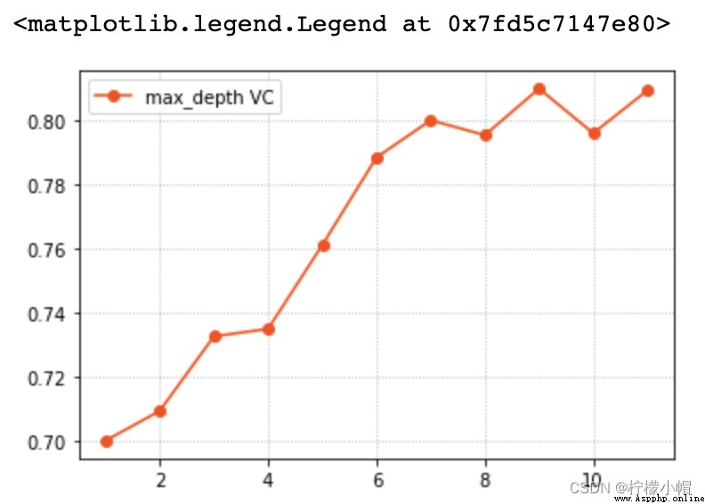
1. Verify the curve
The relationship described by the validation curve is the functional relationship between the model performance and the model hyperparameters :
Model performance = f( Hyperparameters )
2. Verify the curve implementation
sklearn Validation curve provided API:
train_scores, test_scores = ms.validation_curve(
model, # Model
Input set , Output set ,
'n_estimators', # Super parameter name
np.arange(50, 550, 50), # Hyperparametric sequence
cv=5 # Fold number
)
return train_scores And test_scores The score matrix is composed of each cross validation result under each super parameter value .
3. Case study : Predict car grade adjustment parameters
import numpy as np
import pandas as pd
data = pd.read_csv('car.txt', header=None) # I don't want to use the first line as the header
# Complete label coding preprocessing for the current group of data
import sklearn.preprocessing as sp
import sklearn.ensemble as se
import sklearn.model_selection as ms
import sklearn.metrics as sm
# Traverse each column of data
train_data = pd.DataFrame([])
encoders = {
}
for col_ind, col_val in data.items():
encoder = sp.LabelEncoder()
train_data[col_ind] = encoder.fit_transform(col_val)
encoders[col_ind] = encoder
# Organize input and output sets
x, y = train_data.iloc[:, :-1], train_data[6]
# Create a classification model ( Parameter value set after parameter adjustment )
model = se.RandomForestClassifier(max_depth=9, n_estimators=140, random_state=7)
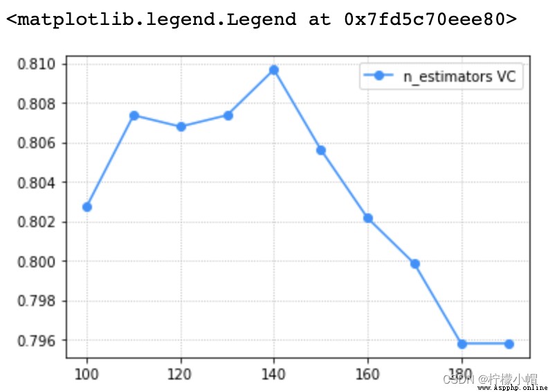
# Verify the curve , Select the optimal hyperparameter
import matplotlib.pyplot as plt
# params = np.arange(50, 550, 50)
params = np.arange(100, 200, 10)
train_scores, test_scores = ms.validation_curve(model, x, y, param_name='n_estimators', param_range=params, cv=5)
scores = test_scores.mean(axis=1)
# Verify curve visualization
plt.grid(linestyle=':')
plt.plot(params, scores, 'o-', color='dodgerblue', label='n_estimators VC')
plt.legend()
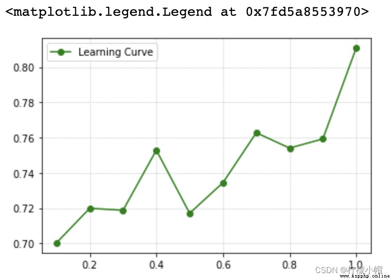
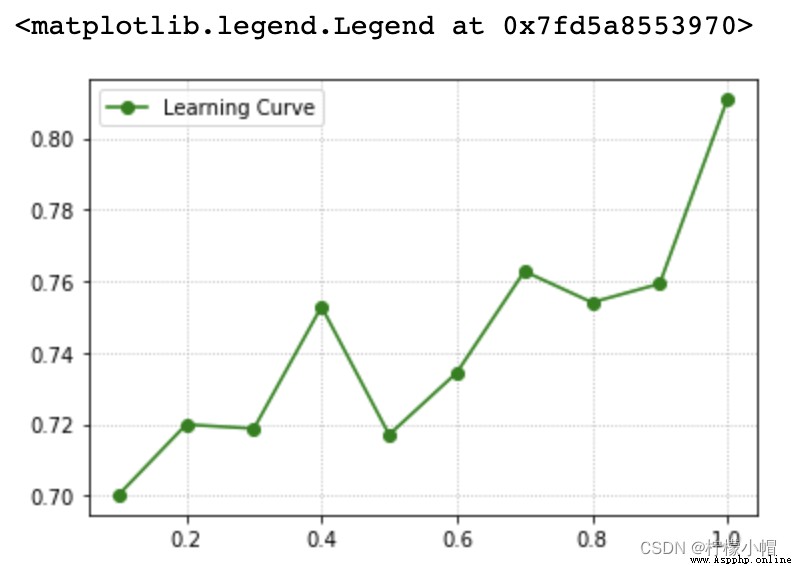
The relationship described by the learning curve is the functional relationship between the model performance and the training sample size :
Model performance = f( Training set size )
5. Learning curve realization
sklearn Learning curve provided API:
train_scores, test_scores = ms.learning_curve(
model, # Model
Input set , Output set ,
train_sizes=[0.9, 0.8, 0.7], # Training set size sequence
cv=5 # Fold number
)
return train_scores And test_scores The score matrix is composed of each cross validation result under each super parameter value .
6. Case study : Predict car grade adjustment parameters
import numpy as np
import pandas as pd
data = pd.read_csv('car.txt', header=None) # I don't want to use the first line as the header
data.head()
""" 0 1 2 3 4 5 6 0 vhigh vhigh 2 2 small low unacc 1 vhigh vhigh 2 2 small med unacc 2 vhigh vhigh 2 2 small high unacc 3 vhigh vhigh 2 2 med low unacc 4 vhigh vhigh 2 2 med med unacc """
# determine : It's about classification , Or the question of return ? classification
# Which classification model to choose : Logical regression 、 Decision tree 、RF、GBDT、AdaBoost? RF
# Complete label coding preprocessing for the current group of data
import sklearn.preprocessing as sp
import sklearn.ensemble as se
import sklearn.model_selection as ms
import sklearn.metrics as sm
# Traverse each column of data
train_data = pd.DataFrame([])
encoders = {
}
for col_ind, col_val in data.items():
encoder = sp.LabelEncoder()
train_data[col_ind] = encoder.fit_transform(col_val)
encoders[col_ind] = encoder
# Organize input and output sets
x, y = train_data.iloc[:, :-1], train_data[6]
# Create a classification model
model = se.RandomForestClassifier(max_depth=9, n_estimators=140, random_state=7)
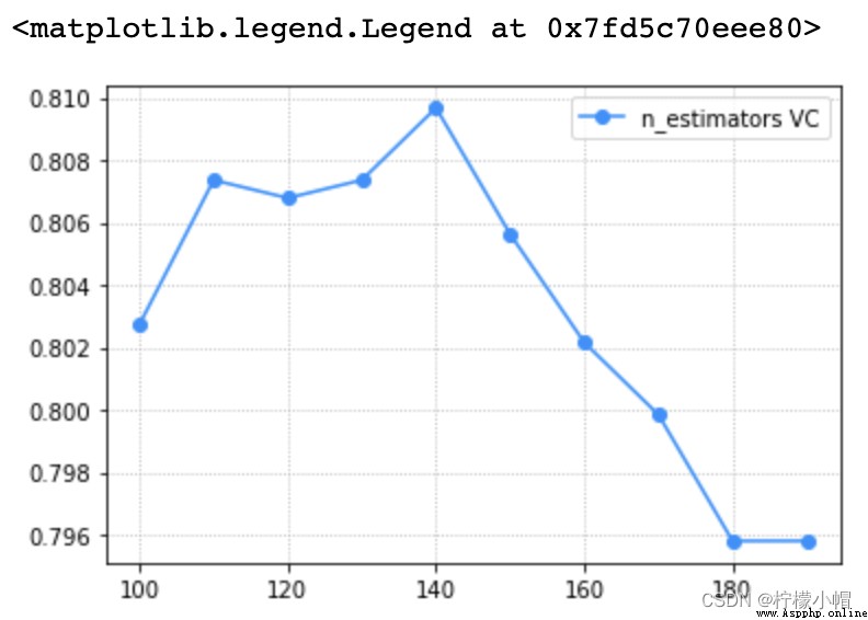
# Verify the curve , Select the optimal hyperparameter
import matplotlib.pyplot as plt
# params = np.arange(50, 550, 50)
params = np.arange(100, 200, 10)
train_scores, test_scores = ms.validation_curve(model, x, y, param_name='n_estimators', param_range=params, cv=5)
scores = test_scores.mean(axis=1)
# Verify curve visualization
plt.grid(linestyle=':')
plt.plot(params, scores, 'o-', color='dodgerblue', label='n_estimators VC')
plt.legend()