Artificial intelligence

Chapter six Support vector machine （ Classification model ）

One 、 Basic concepts

1. What is support vector machine

• “ Support vector machine ”（SVM） It is a supervised machine learning algorithm , It can be used for classification tasks or regression tasks . Mainly used for classification problems . In this algorithm , We plot each data item as n A point in dimensional space （ among n Is the number of features you have ）, The value of each feature is the value of a specific coordinate . then , We perform the classification task by finding the optimal classification hyperplane .
• Support vector machine （Support Vector Machines） It's a two category model , Machine learning 、 Computer vision 、 It is widely used in data mining , It is mainly used to solve the problem of data classification , Its purpose is to find a hyperplane to segment the sample , The principle of segmentation is to maximize the interval （ That is, the distance from the edge point of the dataset to the dividing line d Maximum , Here's the picture ）, Finally, it is transformed into a convex quadratic programming problem . Usually SVM For binary classification problems , For multivariate classification, it can be decomposed into multiple binary classification problems , And then classify . So-called “ Support vector ”, This is the edge point through which the dotted line passes in the figure below . Support vector machine corresponds to the line that can correctly divide the data and has the largest interval （ The red line in the figure below ）.
  

2. Optimal classification boundary

• What is the optimal classification boundary ？ Under what conditions is the classification boundary the optimal boundary ？
  
• As shown in figure of A,B Two sample points ,B The degree of certainty that a point is predicted to be a positive class is greater than A spot , therefore SVM The goal is to find a hyperplane , So that there can be greater spacing between dissimilar points closer to the hyperplane , That is, it is not necessary to consider all sample points , Just let the obtained hyperplane maximize the distance between the points close to it . The hyperplane can be described by the following linear equation ：
  w T x + b = 0 w^T x + b = 0 wTx+b=0
  among , x = ( x 1 ; x 2 ; . . . ; x n ) x=(x_1;x_2;...;x_n) x=(x1​;x2​;...;xn​), w = ( w 1 ; w 2 ; . . . ; w n ) w=(w_1;w_2;...;w_n) w=(w1​;w2​;...;wn​), b b b For the offset term . It can be proved mathematically that , The distance from the support vector to the hyperplane is ：
  γ = 1 ∣ ∣ w ∣ ∣ \gamma = \frac{1}{||w||} γ=∣∣w∣∣1​
  To maximize the distance , Just minimize ∣ ∣ w ∣ ∣ ||w|| ∣∣w∣∣ that will do .

3. SVM Optimal boundary requirements

• SVM When looking for the optimal boundary , The following requirements shall be met ：

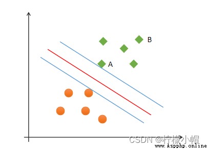
（1） correctness ： Most samples can be classified correctly ;

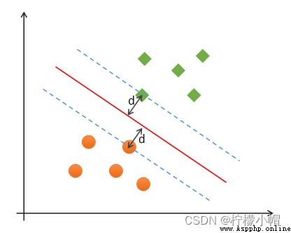
（2） Security ： Support vector , That is, the distance between the samples closest to the classification boundary is the farthest ;

（3） Fairness ： The distance between the support vector and the classification boundary is equal ;

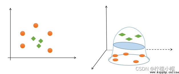
（4） simplicity ： Using linear equations （ A straight line 、 Plane ） Represents the classification boundary , Also called split hyperplane . If linear division cannot be made in the original dimension , Then through the dimension lifting transformation , Seek linear partition hyperplane in higher dimensional space . The transformation from low latitude space to high latitude space is carried out by kernel function .

4. Linearly separable and linearly nonseparable

① Linearly separable

If a set of samples can use a linear function to correctly classify the samples , Call these data samples linearly separable . So what is a linear function ？ It's a straight line in two-dimensional space , It's a plane in three-dimensional space , And so on , If you don't consider the dimension of space , Such linear functions are collectively referred to as hyperplanes .

② Linearly indivisible

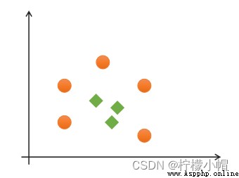
If a set of samples , Unable to find a linear function to correctly classify the samples , These samples are said to be linearly nonseparable . The following is an example of one-dimensional linear indivisibility ：

• The following is an example of two-dimensional indivisibility ：
  
• For this class of linear nonseparable problems , You can upgrade the dimension , The low latitude feature space is mapped to the high latitude feature space , Realize linear separability , As shown in the figure below ：
  

• So how to achieve dimension upgrading ？ This requires the use of kernel functions .

Two 、 The principle of support vector machine

• “ Support vector machine ” The core of the task is ： Find the optimal classification boundary . The optimal classification boundary should have the following characteristics ：
  • correct ： Most samples can be classified correctly .
  • generalization ： Maximize support vector spacing .
  • fair ： Equidistant from the support vector .
  • Simple ： linear , A straight line or plane , hyperplane .

3、 ... and 、 Kernel function of support vector machine

• SVM Through a characteristic transformation called kernel function , New features can be added , It makes the linear nonseparable problem in low dimensional space become linearly separable in high dimensional space .
• If a low dimensional space exists K(x,y),x,y∈Χ, bring K(x,y)=ϕ(x)·ϕ(y), said K(x,y) It's a kernel function , among ϕ(x)·ϕ(y) by x,y Inner product mapped to feature space ,ϕ(x) by X→H The mapping function of .
• Here are some common kernel functions .

1. Linear kernel function

• Linear kernel function ：linear, Do not promote dimensions through kernel functions , Only the linear classification boundary is found in the original dimension space , It is mainly used for linear separable problems .

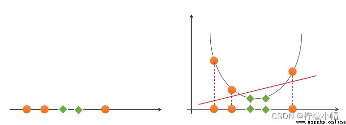
# Support vector machine example 
import numpy as np
import sklearn.model_selection as ms
import sklearn.svm as svm
import sklearn.metrics as sm
import matplotlib.pyplot as mp
x, y = [], []
with open("../data/multiple2.txt", "r") as f:
for line in f.readlines():
data = [float(substr) for substr in line.split(",")]
x.append(data[:-1]) # Input 
y.append(data[-1]) # Output 
# List to array 
x = np.array(x)
y = np.array(y, dtype=int)
# Linear kernel support vector machine classifier 
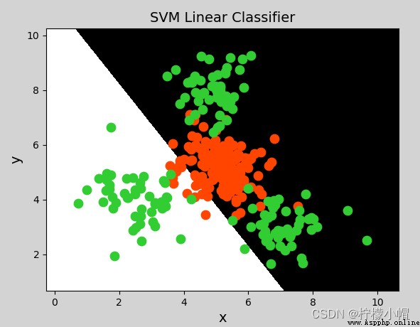
model = svm.SVC(kernel="linear") # Linear kernel function 
# model = svm.SVC(kernel="poly", degree=3) # Polynomial kernel function 
# print("gamma:", model.gamma)
# Radial basis function kernel support vector machine classifier 
# model = svm.SVC(kernel="rbf",
# gamma=0.01, # Standard deviation of probability density 
# C=200) # Probability intensity 
model.fit(x, y)
# Calculate drawing boundaries 
l, r, h = x[:, 0].min() - 1, x[:, 0].max() + 1, 0.005
b, t, v = x[:, 1].min() - 1, x[:, 1].max() + 1, 0.005
# Generate grid matrix 
grid_x = np.meshgrid(np.arange(l, r, h), np.arange(b, t, v))
flat_x = np.c_[grid_x[0].ravel(), grid_x[1].ravel()] # Merge 
flat_y = model.predict(flat_x) # According to the grid matrix prediction classification 
grid_y = flat_y.reshape(grid_x[0].shape) # Restore shape 
mp.figure("SVM Classifier", facecolor="lightgray")
mp.title("SVM Classifier", fontsize=14)
mp.xlabel("x", fontsize=14)
mp.ylabel("y", fontsize=14)
mp.tick_params(labelsize=10)
mp.pcolormesh(grid_x[0], grid_x[1], grid_y, cmap="gray")
C0, C1 = (y == 0), (y == 1)
mp.scatter(x[C0][:, 0], x[C0][:, 1], c="orangered", s=80)
mp.scatter(x[C1][:, 0], x[C1][:, 1], c="limegreen", s=80)
mp.show()

2. Polynomial kernel function

• Polynomial kernel function ：poly, The higher power of the features of the original sample is increased by polynomial function .
• Polynomial kernel function （Polynomial Kernel） Using the method of adding the characteristics of higher-order terms to make dimension lifting transformation , When the polynomial order is high, the complexity will be high , The expression is ：
  K ( x , y ) = ( α x T ⋅ y + c ) d K(x,y)=(αx^T·y+c)d K(x,y)=(αxT⋅y+c)d

y = x 1 + x 2 y = x 1 2 + 2 x 1 x 2 + x 2 2 y = x 1 3 + 3 x 1 2 x 2 + 3 x 1 x 2 2 + x 2 3 y = x_1 + x_2\\ y = x_1^2 + 2x_1x_2+x_2^2\\ y=x_1^3 + 3x_1^2x_2 + 3x_1x_2^2 + x_2^3 y=x1​+x2​y=x12​+2x1​x2​+x22​y=x13​+3x12​x2​+3x1​x22​+x23​

• among ,α Indicates the adjustment parameter ,d Indicates the number of times of the highest order item ,c Is an optional constant .
• Sample code （ Change the support vector machine model created in the previous example to the following code ）：

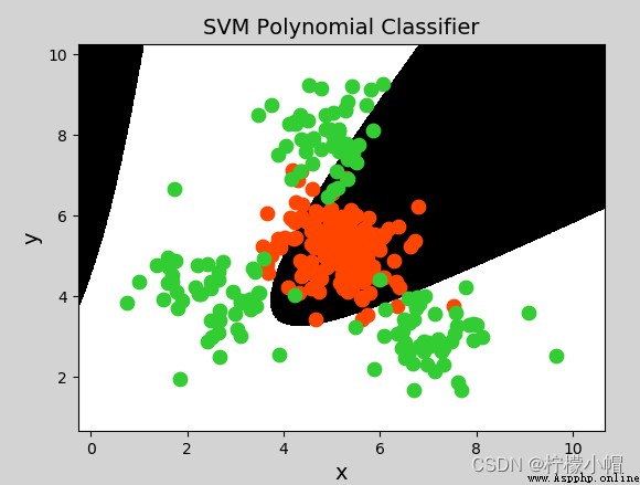
model = svm.SVC(kernel="poly", degree=3) # Polynomial kernel function 

3. Radial basis function

• Radial basis function ：rbf, The Gaussian distribution function is used to increase the distribution probability of the original sample features .
• Radial basis function （Radial Basis Function Kernel） It's very flexible , It's widely used . Compared with polynomial kernel function , It has fewer parameters , So most of the time , They all have better performance . When not sure which kernel function to use , The Gaussian kernel function can be verified first . Because it is similar to Gaussian function , So it is also called Gaussian kernel function .
• Sample code （ Change the classifier model in the previous example to the following code ）：

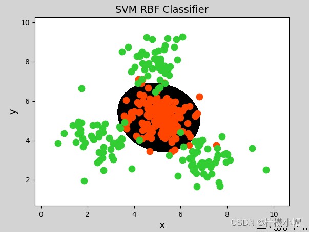
# Radial basis function kernel support vector machine classifier 
model = svm.SVC(kernel="rbf",
gamma=0.01, # Standard deviation of probability density 
C=600) # Probability intensity , The greater the value, the less tolerance for misclassification , The higher the classification accuracy , But the worse the generalization ability ; The smaller the value , The greater the tolerance for misclassification , But the generalization ability is strong 

4. summary

• SVM Linear kernel sklearn The implementation is as follows ：

model = svm.SVC(kernel='linear')
model.fit(train_x, train_y)

• SVM Polynomial kernel function sklearn The implementation is as follows ：

# Support vector machine classifier based on linear kernel function 
model = svm.SVC(kernel='poly', degree=3)
model.fit(train_x, train_y)

• SVM Radial basis kernel function sklearn The implementation is as follows ：

# Support vector machine classifier based on radial basis kernel function 
# C： Regular intensity 
# gamma：'rbf','poly' and 'sigmoid' The kernel function of . The higher the gamma value , The training data set will be accurately fitted , It may lead to over fitting problems .
model = svm.SVC(kernel='rbf', C=600, gamma=0.01)
model.fit(train_x, train_y)

（1） Support vector machine is a binary classification model

（2） Support vector machine finds the optimal linear model as the classification boundary

（3） Boundary requirements ： correctness 、 Fairness 、 Security 、 simplicity

（4） Linear nonseparable problem can be transformed into linear separable problem by kernel function , Kernel functions include ： Linear kernel function 、 Polynomial kernel function 、 Radial basis function

（5） Support vector machine is suitable for the classification of a small number of samples

Four 、 The grid search

• The way to obtain an optimal super parameter can draw the verification curve , However, the verification curve can only obtain one optimal hyperparameter at a time . If there are many permutations and combinations of multiple superparameters , You can use grid search to find the optimal combination of hyperparameters .
• For each super parameter combination in the super parameter combination list , Instantiate a given model , do cv Secondary cross validation , Average them f1 The combination of super parameters with the highest score is the best choice , Instantiate the model object and return .
• Grid search related API：

import sklearn.model_selection as ms
params =
[{
'kernel':['linear'], 'C':[1, 10, 100, 1000]},
{
'kernel':['poly'], 'C':[1], 'degree':[2, 3]},
{
'kernel':['rbf'], 'C':[1,10,100], 'gamma':[1, 0.1, 0.01]}]
model = ms.GridSearchCV( Model , params, cv= Number of cross validation )
model.fit( Input set , Output set )
# Get each parameter combination of grid search 
model.cv_results_['params']
# Get the average test score corresponding to each parameter combination of grid search 
model.cv_results_['mean_test_score']
# Get the best parameters 
model.best_params_
model.best_score_
model.best_estimator_

5、 ... and 、 Case study ： Implementation of support vector machine

import numpy as np
import matplotlib.pyplot as plt
import pandas as pd
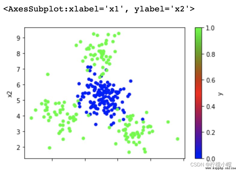
data = pd.read_csv('multiple2.txt', header=None, names=['x1', 'x2', 'y'])
data.plot.scatter(x='x1', y='x2', c='y', cmap='brg')

import sklearn.model_selection as ms
import sklearn.svm as svm
import sklearn.metrics as sm
# Organize data sets , Split test set training set 
x, y = data.iloc[:, :-1], data['y']
train_x, test_x, train_y, test_y = ms.train_test_split(x, y, test_size=0.25, random_state=7)
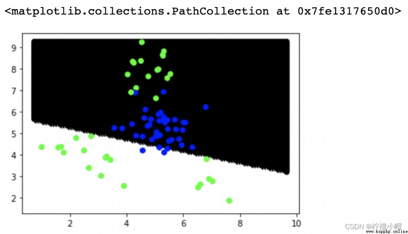
model = svm.SVC(kernel='linear')
model.fit(train_x, train_y)
pred_test_y = model.predict(test_x)
print(sm.classification_report(test_y, pred_test_y))
""" precision recall f1-score support 0 0.69 0.90 0.78 40 1 0.83 0.54 0.66 35 accuracy 0.73 75 macro avg 0.76 0.72 0.72 75 weighted avg 0.75 0.73 0.72 75 """
data.head()
""" x1 x2 y 0 5.35 4.48 0 1 6.72 5.37 0 2 3.57 5.25 0 3 4.77 7.65 1 4 2.25 4.07 1 """

# Violent drawing of classification boundaries 
# from x Of min-max, Dismantle 100 individual x coordinate 
# from y Of min-max, Dismantle 100 individual y coordinate 
# It consists of 10000 Coordinates , Predict the category labels for each coordinate point , Draw a scatter 
xs = np.linspace(data['x1'].min(), data['x1'].max(), 100)
ys = np.linspace(data['x2'].min(), data['x2'].max(), 100)
points = []
for x in xs:
for y in ys:
points.append([x, y])
points = np.array(points)
# Predict the category labels for each coordinate point Draw a scatter 
point_labels = model.predict(points)
plt.scatter(points[:,0], points[:,1], c=point_labels, cmap='gray')
plt.scatter(test_x['x1'], test_x['x2'], c=test_y, cmap='brg')

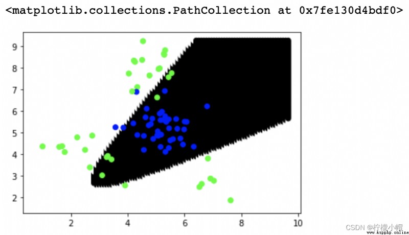
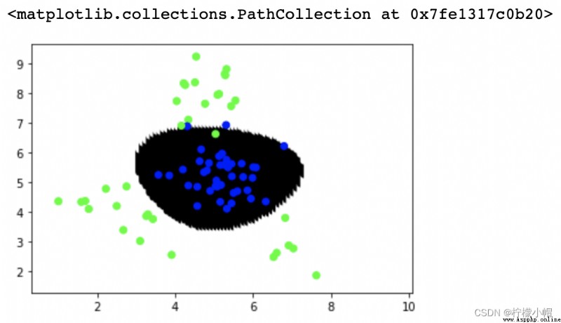
# Polynomial kernel function 
model = svm.SVC(kernel='poly', degree=2)
model.fit(train_x, train_y)
pred_test_y = model.predict(test_x)
print(sm.classification_report(test_y, pred_test_y))
# Predict the category labels for each coordinate point Draw a scatter 
point_labels = model.predict(points)
plt.scatter(points[:,0], points[:,1], c=point_labels, cmap='gray')
plt.scatter(test_x['x1'], test_x['x2'], c=test_y, cmap='brg')
""" precision recall f1-score support 0 0.84 0.95 0.89 40 1 0.93 0.80 0.86 35 accuracy 0.88 75 macro avg 0.89 0.88 0.88 75 weighted avg 0.89 0.88 0.88 75 """

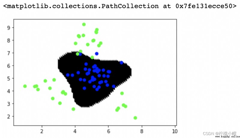
# Radial basis function 
model = svm.SVC(kernel='rbf', C=1, gamma=0.1)
model.fit(train_x, train_y)
pred_test_y = model.predict(test_x)
# print(sm.classification_report(test_y, pred_test_y))
# Predict the category labels for each coordinate point Draw a scatter 
point_labels = model.predict(points)
plt.scatter(points[:,0], points[:,1], c=point_labels, cmap='gray')
plt.scatter(test_x['x1'], test_x['x2'], c=test_y, cmap='brg')
""" precision recall f1-score support 0 0.97 0.97 0.97 40 1 0.97 0.97 0.97 35 accuracy 0.97 75 macro avg 0.97 0.97 0.97 75 weighted avg 0.97 0.97 0.97 75 """

# The optimal combination of super parameters is found by grid search 
model = svm.SVC()
# The grid search 
params = [{
'kernel':['linear'], 'C':[1, 10, 100]},
{
'kernel':['poly'], 'degree':[2, 3]},
{
'kernel':['rbf'], 'C':[1, 10, 100], 'gamma':[1, 0.1, 0.001]}]
model = ms.GridSearchCV(model, params, cv=5)
model.fit(train_x, train_y)
pred_test_y = model.predict(test_x)
# print(sm.classification_report(test_y, pred_test_y))
# Predict the category labels for each coordinate point Draw a scatter 
point_labels = model.predict(points)
plt.scatter(points[:,0], points[:,1], c=point_labels, cmap='gray')
plt.scatter(test_x['x1'], test_x['x2'], c=test_y, cmap='brg')

print(model.best_params_)
print(model.best_score_)
print(model.best_estimator_)
""" {'C': 1, 'gamma': 1, 'kernel': 'rbf'} 0.9511111111111111 SVC(C=1, gamma=1) """