1. Theoretical basis of image pyramid
2. Down sampling function and use
3. Upward sampling function and its application
4. Study on sampling reversibility
5. The pyramid of Laplace
6. Image outline introduction
The outline is approximate
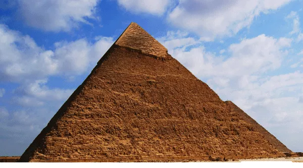
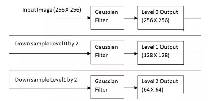
Image pyramid is a kind of multi-scale expression of image , It is an effective but simple concept structure for interpreting images at multi-resolution . The pyramid of an image is a series of pyramid shaped pyramids with gradually decreasing resolution , And from the same original image set . It is obtained by step down sampling , Stop sampling until a certain termination condition is reached . We compare layers of images to pyramids , The higher the level , The smaller the image , Lower resolution .
Then why should we make an image pyramid ? This is because changing the pixel size sometimes does not change its characteristics , Let's show you 1000 Megapixel image , You know there's someone inside , I'll show you a 100000 pixel , You can also know there's someone inside , But for computers , Processing 100000 pixels, comparable processing 1000 Ten thousand pixels is much easier . To make it easier for computers to recognize features , Later, we will also talk about the practical project of feature recognition , Maybe you played basketball in high school , I saw your head teacher coming out from afar , You leave 500 rice , You can still recognize your teachers by their characteristics , Leave you with your head teacher 2 It's the same with rice .
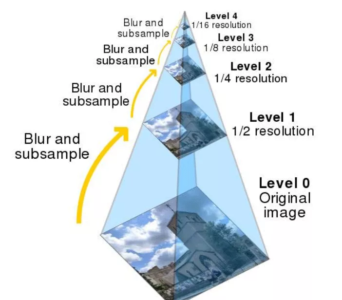
in other words Image pyramid a collection of subgraphs with different resolutions of the same image . Here we can give an example that the original image is a 400400 Image , Then take it up and it will be 200200 And then 100*100, This reduces the resolution , But it's always the same image .
So from the first i Layer to tier i+1 layer , How exactly did he do it ?
1. Calculate the approximate value of the reduced resolution of the input image . This can be done by filtering the input and 2 Sample for step size ( Subsampling ). There are many filtering operations that can be used , Such as neighborhood average ( The average pyramid can be generated ), Gaussian low pass filter ( Gaussian pyramid can be generated ), Or no filtering , Generate sub sampling pyramid . The quality of the generated approximation is a function of the selected filter . No filter , The confusion in the upper layer of the pyramid becomes obvious , The sub sampling points are not very representative of the selected area .
2. Interpolate the output from the previous step ( The factor is still 2) And filter it . This will generate a predictive image with the same resolution as the input . Because in step 1 Interpolation between the output pixels of , So the insertion filter determines the predicted value and the steps 1 The degree of approximation between the inputs of . If the insertion filter is ignored , Then the predicted value will be step 1 Interpolation form of output , The block effect of duplicate pixels will become obvious .
3. computational procedure 2 The predicted values and steps 1 The difference between the inputs of . With j The difference identified by the level prediction residual will be used for the reconstruction of the original image . Without quantifying the difference , The prediction residual pyramid can be used to generate the corresponding approximate pyramid ( Including the original image ), Without error .
Perform the above process P Times will produce closely related P+1 First order approximation and prediction residual pyramid .j-1 The output of the first approximation is used to provide an approximation pyramid , and j The output of level prediction residuals is placed in the prediction residuals pyramid . If you don't need a prediction residual pyramid , Then step 2 and 3、 Interpolator 、 The insertion filter and the adder in the figure can be omitted .
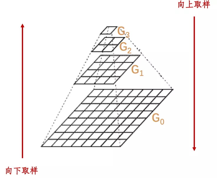
Here, down sampling represents the reduction of the image . Upsampling indicates an increase in image size .
1. To image Gi Gaussian kernel convolution .
Gaussian kernel convolution is what we call Gaussian filter manipulation , We have already talked about , Use a Gaussian convolution kernel , Let the adjacent pixel value take a larger weight , Then do relevant operations with the target image .
2. Delete all even rows and columns .
original image M * N Processing results M/2 * N/2. After each treatment , The resulting image is the original 1/4. This operation is called Octave. Repeat the process , Construct image pyramids . Until the image can not be further divided . This process will lose image information .
Sampling upward is just the opposite of sampling downward , On the original image ,** Expand into the original in each direction 2 times , New rows and columns with 0 fill . Use with “ Use... Downward ” The same convolution kernel times 4, obtain “ New pixels ” The new value of .** The image will be blurred after upward sampling .
Sampling up 、 Down sampling is not an inverse operation . After two operations , Unable to restore the original image .
Image pyramid down sampling function :
dst=cv2.pyrDown(src)import cv2import numpy as npo=cv2.imread("image\\man.bmp")r1=cv2.pyrDown(o)r2=cv2.pyrDown(r1)r3=cv2.pyrDown(r2)cv2.imshow("original",o)cv2.imshow("PyrDown1",r1)cv2.imshow("PyrDown2",r2)cv2.imshow("PyrDown3",r3)cv2.waitKey()cv2.destroyAllWindows()Here we do three down sampling on the image , The result is :
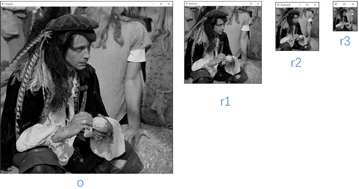
Down sampling will lose information !!!
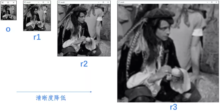
3. Upward sampling function and its applicationImage pyramid up sampling function :
dst=cv2.pyrUp(src)We won't introduce the code here .
Take a look at our results directly :
Here, let's take a look at the image after sampling downward and then sampling upward , Is it consistent . There is also the image sampling upward and then downward , Are they consistent ? Here we do some research with the image of a little girl .
First of all, let's analyze it : When the image is sampled down once , Image by MN Turned into M/2N/2, Then, after upward sampling again, it becomes M*N. So it can be proved that for the picture size It doesn't change .
import cv2o=cv2.imread("image\\girl.bmp")down=cv2.pyrDown(o)up=cv2.pyrUp(down)cv2.imshow("original",o)cv2.imshow("down",down)cv2.imshow("up",up)cv2.waitKey()cv2.destroyAllWindows()So let's see what has changed ?
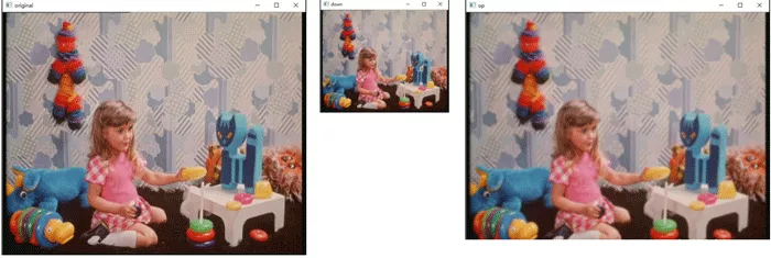
It can be clearly seen here that the picture of the little girl has become blurred , So why ? Because as we mentioned above, when the image becomes smaller , Then you will lose some information , After zooming in again , Because the convolution kernel gets bigger , Then the image will become blurred . So it will not be consistent with the original image .
Then let's take a look at the upward sampling operation first , What would it look like to do a downward sampling operation ? Since the image becomes too large, we omit the image sampled upward from the intermediate image .
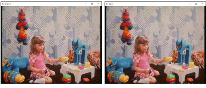
Then it is not particularly easy for us to find differences with the naked eye , So let's use image subtraction to see .
import cv2o=cv2.imread("image\\girl.bmp")up=cv2.pyrUp(o)down=cv2.pyrDown(up)diff=down-o # structure diff Images , see down And o The difference between cv2.imshow("difference",diff)cv2.waitKey()cv2.destroyAllWindows()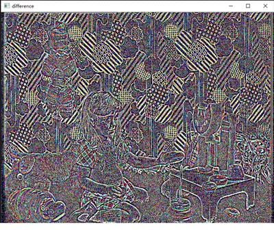
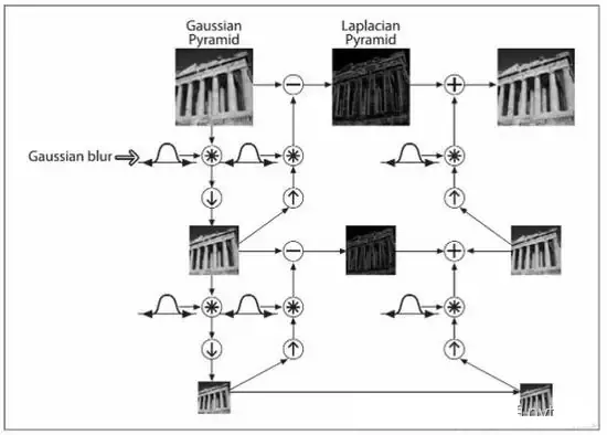
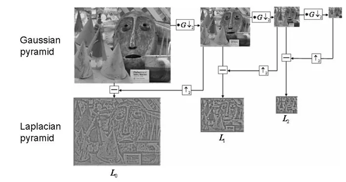
Let's first look at what the Laplace pyramid is :
Li = Gi - PyrUp(PyrDown(Gi))
We can know from his formula , Laplacian pyramid is a process of subtracting downward sampling from the original image and then upward sampling .
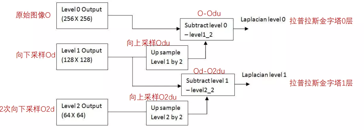
Displayed in the image is :
The core function is :
od=cv2.pyrDown(o)odu=cv2.pyrUp(od)lapPyr=o-odu6. Image outline introduction First of all, we need to explain that the contour of the image is different from the edge of the image , The edges are scattered , But the outline is a whole .
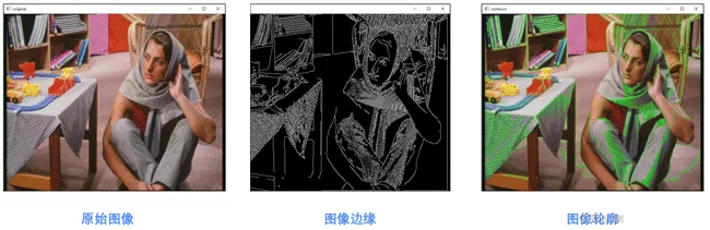
Edge detection can detect edges , But the edges are discontinuous . Connect the edges as a whole , Form an outline .
Be careful :
The object is a binary image . Therefore, it is necessary to perform threshold segmentation or edge detection in advance . Finding the contour requires changing the original image . therefore , Usually a copy of the original image is used . stay OpenCV in , Is to find white objects from a black background . therefore , The object must be white , The background must be black .
For the detection of image contour, the required function is :
cv2.findContours( ) and cv2.drawContours( )
The function to find the image outline is cv2.findContours(), adopt cv2.drawContours() Draw the found contour onto the image .
about cv2.findContours( ) function :
image, contours, hierarchy = cv2.findContours( image, mode, method)
Note here that in the latest version , There are only two return functions in the contour :
contours, hierarchy = cv2.findContours( image, mode, method)
contours , outline
hierarchy , The topological information of the image ( Contour hierarchy )
image , original image
mode , Contour retrieval mode
method , The approximate method of contour
Here we need to introduce mode: That is, contour retrieval mode :
cv2.RETR_EXTERNAL : Indicates that only the outer contour is detected
cv2.RETR_LIST : The detected contour does not establish a hierarchical relationship
cv2.RETR_CCOMP : Build two levels of outline , The upper layer is the outer boundary , The inner layer is the edge of the inner hole Boundary information . If there is another hole in the inner hole
Connected objects , The boundary of this object is also at the top
cv2.RETR_TREE : Create a hierarchical tree structure outline .
Then let's introduce method , The approximate method of contour :
cv2.CHAIN_APPROX_NONE : Store all contour points , The pixel position difference between two adjacent points shall not exceed 1, namely max(abs(x1-x2),abs(y2-y1))==1
cv2.CHAIN_APPROX_SIMPLE: Compress the horizontal direction , vertical direction , Diagonal elements , Only the coordinates of the end point in this direction are reserved , For example, a rectangular outline only needs 4 Points to save profile information
cv2.CHAIN_APPROX_TC89_L1: Use teh-Chinl chain The approximate algorithm
cv2.CHAIN_APPROX_TC89_KCOS: Use teh-Chinl chain The approximate algorithm
For example, do contour detection for a rectangle , Use cv2.CHAIN_APPROX_NONE and cv2.CHAIN_APPROX_SIMPLE The result is :
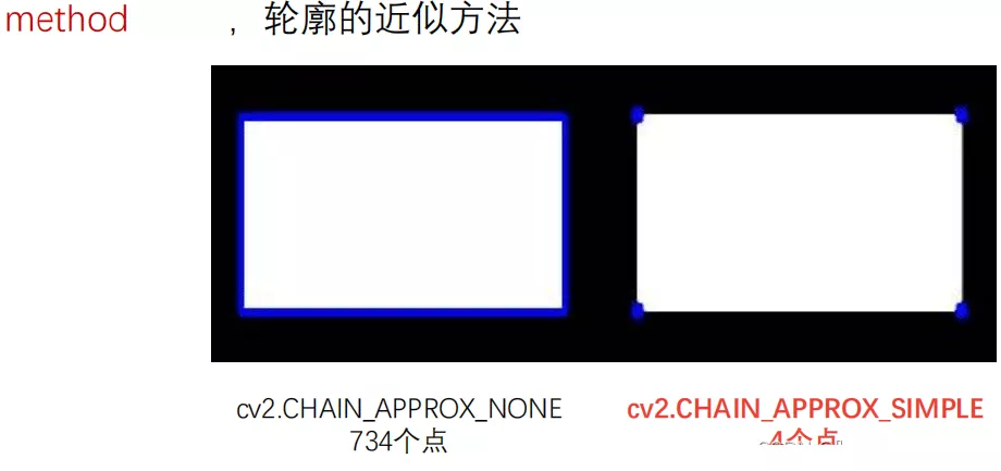
It can be seen that the latter saves a lot of computing space .
about cv2.drawContours( ):
r=cv2.drawContours(o, contours, contourIdx, color[, thickness])
r : Target image , Directly modify the pixels of the target , Implement drawing .
o : original image
contours : The edge array that needs to be drawn .
contourIdx : The edge index that needs to be drawn , If all are drawn, it is -1.
color : The color of the painting , by BGR Format Scalar .
thickness : Optional , Plotted density , That is, the thickness of the brush used to draw the outline .
import cv2import numpy as npo = cv2.imread('image\\boyun.png') gray = cv2.cvtColor(o,cv2.COLOR_BGR2GRAY) ret, binary = cv2.threshold(gray,127,255,cv2.THRESH_BINARY) image,contours, hierarchy =cv2.findContours(binary,cv2.RETR_TREE, cv2.CHAIN_APPROX_SIMPLE) co=o.copy()r=cv2.drawContours(co,contours,-1,(0,0,255),1) cv2.imshow("original",o)cv2.imshow("result",r)cv2.waitKey()cv2.destroyAllWindows()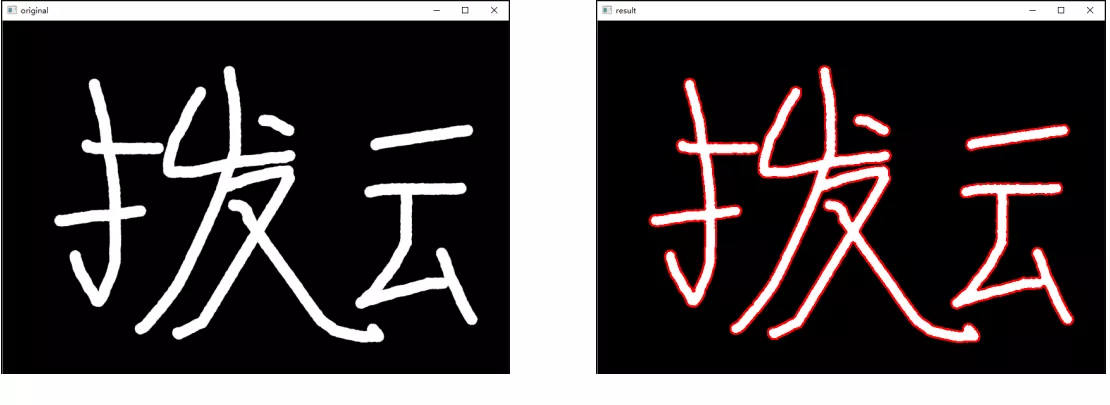
For multiple profiles , We can also specify which outline to draw .
gray = cv2.cvtColor(o,cv2.COLOR_BGR2GRAY) ret, binary = cv2.threshold(gray,127,255,cv2.THRESH_BINARY) image,contours, hierarchy = cv2.findContours(binary,cv2.RETR_TREE,cv2.CHAIN_APPROX_SIMPLE) co=o.copy()r=cv2.drawContours(co,contours,0,(0,0,255),6)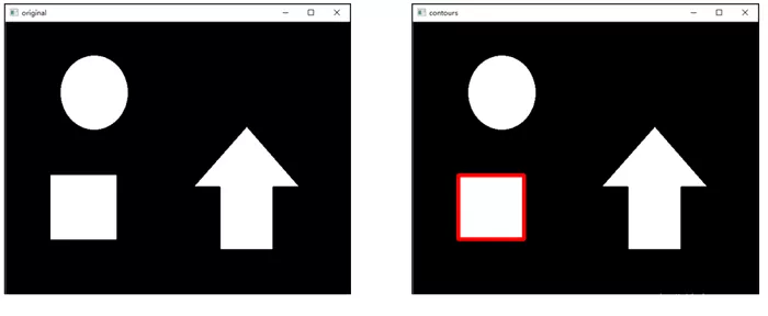
If I set it to -1, Then it is all displayed !!!
The outline is approximateWhen there are burrs in the contour , We want to be able to do contour approximation , Remove burrs , The general idea is to replace the curve with a straight line , But there is a length threshold that needs to be set by yourself .
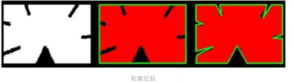
We can also do additional operations , For example, circumscribed rectangle , Circumcircle , Outer ellipse, etc .
img = cv2.imread('contours.png')gray = cv2.cvtColor(img, cv2.COLOR_BGR2GRAY)ret, thresh = cv2.threshold(gray, 127, 255, cv2.THRESH_BINARY)binary, contours, hierarchy = cv2.findContours(thresh, cv2.RETR_TREE, cv2.CHAIN_APPROX_NONE)cnt = contours[0]x,y,w,h = cv2.boundingRect(cnt)img = cv2.rectangle(img,(x,y),(x+w,y+h),(0,255,0),2)cv_show(img,'img')area = cv2.contourArea(cnt)x, y, w, h = cv2.boundingRect(cnt)rect_area = w * hextent = float(area) / rect_areaprint (' The ratio of contour area to boundary rectangle ',extent) Circumcircle (x,y),radius = cv2.minEnclosingCircle(cnt)center = (int(x),int(y))radius = int(radius)img = cv2.circle(img,center,radius,(0,255,0),2)cv_show(img,'img')Template matching is very similar to convolution , The template slides from the origin on the original image , Computing templates and ( Where the image is covered by the template ) The degree of difference , The calculation of the degree of difference is in opencv There are six in the , Then put the results of each calculation into a matrix , Output as a result . If the original figure is AXB size , And the template is axb size , Then the output matrix is (A-a+1)x(B-b+1).
TM_SQDIFF: The square is different , The smaller the calculated value , The more relevant
TM_CCORR: Calculate correlation , The larger the calculated value , The more relevant
TM_CCOEFF: Calculate the correlation coefficient , The larger the calculated value , The more relevant
TM_SQDIFF_NORMED: Calculating the normalized square is different , The closer the calculated value is to 0, The more relevant
TM_CCORR_NORMED: Calculate the normalized correlation , The closer the calculated value is to 1, The more relevant
TM_CCOEFF_NORMED: Calculate the normalized correlation coefficient , The closer the calculated value is to 1, The more relevant

This is about python OpenCV This is the end of the article on image pyramid , More about python OpenCV Please search the previous articles of SDN or continue to browse the related articles below. I hope you will support SDN more in the future !