One 、 Overview of monocular 3D reconstruction
Two 、 Implementation process
(1) Camera calibration
(2) Image feature extraction and matching
(3) Three dimensional reconstruction
3、 ... and 、 Conclusion
Four 、 Code
summary
One 、 Overview of monocular 3D reconstructionThe object of the objective world is three-dimensional , And the image we get with the camera is two-dimensional , But we can perceive the three-dimensional information of the target through the two-dimensional image . 3D reconstruction technology is to process images in a certain way and then obtain 3D information that can be recognized by computer , Therefore, the target is analyzed . The reconstruction is based on the motion of a single binocular camera , So as to obtain the three-dimensional visual information of the object in space , among , Monocular refers to a single camera .
Two 、 Implementation processIn the process of monocular three-dimensional reconstruction of objects , The relevant operating environment is as follows :
matplotlib 3.3.4
numpy 1.19.5
opencv-contrib-python 3.4.2.16
opencv-python 3.4.2.16
pillow 8.2.0
python 3.6.2
Its reconstruction mainly includes the following steps :
(1) Camera calibration
(2) Image feature extraction and matching
(3) Three dimensional reconstruction
Next , Let's take a detailed look at the specific implementation of each step :
(1) Camera calibrationThere are many cameras in our daily life , Such as the camera on the mobile phone 、 Digital camera and function module camera, etc , The parameters of each camera are different , That is, the resolution of the photos taken by the camera 、 Patterns, etc . Suppose we are doing three-dimensional reconstruction of an object , We don't know the matrix parameters of our camera in advance , that , We should calculate the matrix parameters of the camera , This step is called camera calibration . I won't introduce the relevant principles of camera calibration , Many people on the Internet explained it in detail . The specific implementation of its calibration is as follows :
def camera_calibration(ImagePath): # Cycle break criteria = (cv2.TERM_CRITERIA_EPS + cv2.TERM_CRITERIA_MAX_ITER, 30, 0.001) # Chessboard size ( The number of intersections of the chessboard ) row = 11 column = 8 objpoint = np.zeros((row * column, 3), np.float32) objpoint[:, :2] = np.mgrid[0:row, 0:column].T.reshape(-1, 2) objpoints = [] # 3d point in real world space imgpoints = [] # 2d points in image plane. batch_images = glob.glob(ImagePath + '/*.jpg') for i, fname in enumerate(batch_images): img = cv2.imread(batch_images[i]) imgGray = cv2.cvtColor(img, cv2.COLOR_BGR2GRAY) # find chess board corners ret, corners = cv2.findChessboardCorners(imgGray, (row, column), None) # if found, add object points, image points (after refining them) if ret: objpoints.append(objpoint) corners2 = cv2.cornerSubPix(imgGray, corners, (11, 11), (-1, -1), criteria) imgpoints.append(corners2) # Draw and display the corners img = cv2.drawChessboardCorners(img, (row, column), corners2, ret) cv2.imwrite('Checkerboard_Image/Temp_JPG/Temp_' + str(i) + '.jpg', img) print(" Successfully extracted :", len(batch_images), " Corner of picture !") ret, mtx, dist, rvecs, tvecs = cv2.calibrateCamera(objpoints, imgpoints, imgGray.shape[::-1], None, None)among ,cv2.calibrateCamera Function mtx The matrix is K matrix .
After modifying the corresponding parameters and completing the calibration , We can output the corner picture of the chessboard to see if the corner of the chessboard has been successfully extracted , The output corner diagram is as follows :
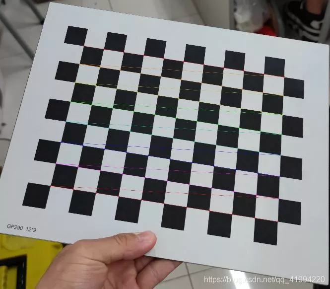
chart 1: Checkerboard corner extraction
(2) Image feature extraction and matching In the whole process of 3D reconstruction , This is the most critical step , And the most complicated step , The quality of image feature extraction determines your final reconstruction effect .
In the image feature point extraction algorithm , Three algorithms are commonly used , Respectively :SIFT Algorithm 、SURF Algorithm and ORB Algorithm . Through comprehensive analysis and comparison , In this step, we take SURF Algorithm to extract the feature points of the picture . Comparison of feature point extraction effects of the three algorithms. If you are interested, you can search online , I won't compare them one by one . The specific implementation is as follows :
def epipolar_geometric(Images_Path, K): IMG = glob.glob(Images_Path) img1, img2 = cv2.imread(IMG[0]), cv2.imread(IMG[1]) img1_gray = cv2.cvtColor(img1, cv2.COLOR_BGR2GRAY) img2_gray = cv2.cvtColor(img2, cv2.COLOR_BGR2GRAY) # Initiate SURF detector SURF = cv2.xfeatures2d_SURF.create() # compute keypoint & descriptions keypoint1, descriptor1 = SURF.detectAndCompute(img1_gray, None) keypoint2, descriptor2 = SURF.detectAndCompute(img2_gray, None) print(" Number of corners :", len(keypoint1), len(keypoint2)) # Find point matches bf = cv2.BFMatcher(cv2.NORM_L2, crossCheck=True) matches = bf.match(descriptor1, descriptor2) print(" Number of matching points :", len(matches)) src_pts = np.asarray([keypoint1[m.queryIdx].pt for m in matches]) dst_pts = np.asarray([keypoint2[m.trainIdx].pt for m in matches]) # plot knn_image = cv2.drawMatches(img1_gray, keypoint1, img2_gray, keypoint2, matches[:-1], None, flags=2) image_ = Image.fromarray(np.uint8(knn_image)) image_.save("MatchesImage.jpg") # Constrain matches to fit homography retval, mask = cv2.findHomography(src_pts, dst_pts, cv2.RANSAC, 100.0) # We select only inlier points points1 = src_pts[mask.ravel() == 1] points2 = dst_pts[mask.ravel() == 1]The feature points found are as follows :
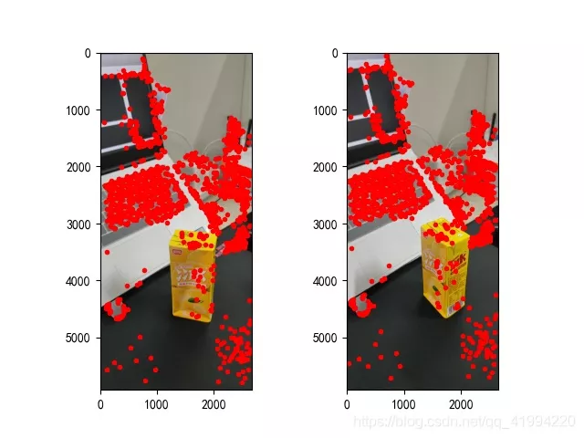
chart 2: Feature point extraction
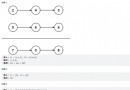
(3) Three dimensional reconstructionAfter we find the feature points of the picture and match each other , You can start 3D reconstruction , The specific implementation is as follows :
points1 = cart2hom(points1.T)points2 = cart2hom(points2.T)# plotfig, ax = plt.subplots(1, 2)ax[0].autoscale_view('tight')ax[0].imshow(cv2.cvtColor(img1, cv2.COLOR_BGR2RGB))ax[0].plot(points1[0], points1[1], 'r.')ax[1].autoscale_view('tight')ax[1].imshow(cv2.cvtColor(img2, cv2.COLOR_BGR2RGB))ax[1].plot(points2[0], points2[1], 'r.')plt.savefig('MatchesPoints.jpg')fig.show()# points1n = np.dot(np.linalg.inv(K), points1)points2n = np.dot(np.linalg.inv(K), points2)E = compute_essential_normalized(points1n, points2n)print('Computed essential matrix:', (-E / E[0][1]))P1 = np.array([[1, 0, 0, 0], [0, 1, 0, 0], [0, 0, 1, 0]])P2s = compute_P_from_essential(E)ind = -1for i, P2 in enumerate(P2s): # Find the correct camera parameters d1 = reconstruct_one_point(points1n[:, 0], points2n[:, 0], P1, P2) # Convert P2 from camera view to world view P2_homogenous = np.linalg.inv(np.vstack([P2, [0, 0, 0, 1]])) d2 = np.dot(P2_homogenous[:3, :4], d1) if d1[2] > 0 and d2[2] > 0: ind = iP2 = np.linalg.inv(np.vstack([P2s[ind], [0, 0, 0, 1]]))[:3, :4]Points3D = linear_triangulation(points1n, points2n, P1, P2)fig = plt.figure()fig.suptitle('3D reconstructed', fontsize=16)ax = fig.gca(projection='3d')ax.plot(Points3D[0], Points3D[1], Points3D[2], 'b.')ax.set_xlabel('x axis')ax.set_ylabel('y axis')ax.set_zlabel('z axis')ax.view_init(elev=135, azim=90)plt.savefig('Reconstruction.jpg')plt.show()The reconstruction effect is as follows ( Results the general ):
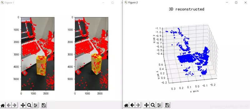
chart 3: Three dimensional reconstruction
3、 ... and 、 ConclusionFrom the results of reconstruction , The effect of monocular 3D reconstruction is general , I think it may be related to these factors :
(1) Picture shooting form . If it is a monocular 3D reconstruction task , When taking pictures, it's best to keep moving the camera in parallel , And it's best to shoot directly , That is, don't shoot sideways or from a different angle ;
(2) When shooting, the surrounding environment interferes . It's best to choose a single place to shoot , Reduce the interference of irrelevant objects ;
(3) Shooting light source problem . The selected photographing site should ensure appropriate brightness ( Specific circumstances need to try to know whether your light source meets the standard ), In addition, when moving the camera, it is also necessary to ensure the consistency of the light source of the previous moment and this moment .
Actually , The effect of monocular 3D reconstruction is really average , Even if all aspects of the situation are full , The reconstruction effect may not be particularly good . Or we can consider using binocular 3D reconstruction , The effect of three-dimensional reconstruction is better than that of binocular reconstruction , In the implementation, it is troublesome ( Billion ) A little , ha-ha . In fact, there are not many operations , It's mainly the trouble of shooting and calibrating two cameras with the whole two cameras , Everything else is fine .
Four 、 Code All the codes of this experiment are as follows :
GitHub:https://github.com/DeepVegChicken/Learning-3DReconstruction
import cv2import jsonimport numpy as npimport globfrom PIL import Imageimport matplotlib.pyplot as pltplt.rcParams['font.sans-serif'] = ['SimHei']plt.rcParams['axes.unicode_minus'] = Falsedef cart2hom(arr): """ Convert catesian to homogenous points by appending a row of 1s :param arr: array of shape (num_dimension x num_points) :returns: array of shape ((num_dimension+1) x num_points) """ if arr.ndim == 1: return np.hstack([arr, 1]) return np.asarray(np.vstack([arr, np.ones(arr.shape[1])]))def compute_P_from_essential(E): """ Compute the second camera matrix (assuming P1 = [I 0]) from an essential matrix. E = [t]R :returns: list of 4 possible camera matrices. """ U, S, V = np.linalg.svd(E) # Ensure rotation matrix are right-handed with positive determinant if np.linalg.det(np.dot(U, V)) < 0: V = -V # create 4 possible camera matrices (Hartley p 258) W = np.array([[0, -1, 0], [1, 0, 0], [0, 0, 1]]) P2s = [np.vstack((np.dot(U, np.dot(W, V)).T, U[:, 2])).T, np.vstack((np.dot(U, np.dot(W, V)).T, -U[:, 2])).T, np.vstack((np.dot(U, np.dot(W.T, V)).T, U[:, 2])).T, np.vstack((np.dot(U, np.dot(W.T, V)).T, -U[:, 2])).T] return P2sdef correspondence_matrix(p1, p2): p1x, p1y = p1[:2] p2x, p2y = p2[:2] return np.array([ p1x * p2x, p1x * p2y, p1x, p1y * p2x, p1y * p2y, p1y, p2x, p2y, np.ones(len(p1x)) ]).T return np.array([ p2x * p1x, p2x * p1y, p2x, p2y * p1x, p2y * p1y, p2y, p1x, p1y, np.ones(len(p1x)) ]).Tdef scale_and_translate_points(points): """ Scale and translate image points so that centroid of the points are at the origin and avg distance to the origin is equal to sqrt(2). :param points: array of homogenous point (3 x n) :returns: array of same input shape and its normalization matrix """ x = points[0] y = points[1] center = points.mean(axis=1) # mean of each row cx = x - center[0] # center the points cy = y - center[1] dist = np.sqrt(np.power(cx, 2) + np.power(cy, 2)) scale = np.sqrt(2) / dist.mean() norm3d = np.array([ [scale, 0, -scale * center[0]], [0, scale, -scale * center[1]], [0, 0, 1] ]) return np.dot(norm3d, points), norm3ddef compute_image_to_image_matrix(x1, x2, compute_essential=False): """ Compute the fundamental or essential matrix from corresponding points (x1, x2 3*n arrays) using the 8 point algorithm. Each row in the A matrix below is constructed as [x'*x, x'*y, x', y'*x, y'*y, y', x, y, 1] """ A = correspondence_matrix(x1, x2) # compute linear least square solution U, S, V = np.linalg.svd(A) F = V[-1].reshape(3, 3) # constrain F. Make rank 2 by zeroing out last singular value U, S, V = np.linalg.svd(F) S[-1] = 0 if compute_essential: S = [1, 1, 0] # Force rank 2 and equal eigenvalues F = np.dot(U, np.dot(np.diag(S), V)) return Fdef compute_normalized_image_to_image_matrix(p1, p2, compute_essential=False): """ Computes the fundamental or essential matrix from corresponding points using the normalized 8 point algorithm. :input p1, p2: corresponding points with shape 3 x n :returns: fundamental or essential matrix with shape 3 x 3 """ n = p1.shape[1] if p2.shape[1] != n: raise ValueError('Number of points do not match.') # preprocess image coordinates p1n, T1 = scale_and_translate_points(p1) p2n, T2 = scale_and_translate_points(p2) # compute F or E with the coordinates F = compute_image_to_image_matrix(p1n, p2n, compute_essential) # reverse preprocessing of coordinates # We know that P1' E P2 = 0 F = np.dot(T1.T, np.dot(F, T2)) return F / F[2, 2]def compute_fundamental_normalized(p1, p2): return compute_normalized_image_to_image_matrix(p1, p2)def compute_essential_normalized(p1, p2): return compute_normalized_image_to_image_matrix(p1, p2, compute_essential=True)def skew(x): """ Create a skew symmetric matrix *A* from a 3d vector *x*. Property: np.cross(A, v) == np.dot(x, v) :param x: 3d vector :returns: 3 x 3 skew symmetric matrix from *x* """ return np.array([ [0, -x[2], x[1]], [x[2], 0, -x[0]], [-x[1], x[0], 0] ])def reconstruct_one_point(pt1, pt2, m1, m2): """ pt1 and m1 * X are parallel and cross product = 0 pt1 x m1 * X = pt2 x m2 * X = 0 """ A = np.vstack([ np.dot(skew(pt1), m1), np.dot(skew(pt2), m2) ]) U, S, V = np.linalg.svd(A) P = np.ravel(V[-1, :4]) return P / P[3]def linear_triangulation(p1, p2, m1, m2): """ Linear triangulation (Hartley ch 12.2 pg 312) to find the 3D point X where p1 = m1 * X and p2 = m2 * X. Solve AX = 0. :param p1, p2: 2D points in homo. or catesian coordinates. Shape (3 x n) :param m1, m2: Camera matrices associated with p1 and p2. Shape (3 x 4) :returns: 4 x n homogenous 3d triangulated points """ num_points = p1.shape[1] res = np.ones((4, num_points)) for i in range(num_points): A = np.asarray([ (p1[0, i] * m1[2, :] - m1[0, :]), (p1[1, i] * m1[2, :] - m1[1, :]), (p2[0, i] * m2[2, :] - m2[0, :]), (p2[1, i] * m2[2, :] - m2[1, :]) ]) _, _, V = np.linalg.svd(A) X = V[-1, :4] res[:, i] = X / X[3] return resdef writetofile(dict, path): for index, item in enumerate(dict): dict[item] = np.array(dict[item]) dict[item] = dict[item].tolist() js = json.dumps(dict) with open(path, 'w') as f: f.write(js) print(" Parameters have been successfully saved to file ")def readfromfile(path): with open(path, 'r') as f: js = f.read() mydict = json.loads(js) print(" Parameter reading succeeded ") return mydictdef camera_calibration(SaveParamPath, ImagePath): # Cycle break criteria = (cv2.TERM_CRITERIA_EPS + cv2.TERM_CRITERIA_MAX_ITER, 30, 0.001) # Chessboard size row = 11 column = 8 objpoint = np.zeros((row * column, 3), np.float32) objpoint[:, :2] = np.mgrid[0:row, 0:column].T.reshape(-1, 2) objpoints = [] # 3d point in real world space imgpoints = [] # 2d points in image plane. batch_images = glob.glob(ImagePath + '/*.jpg') for i, fname in enumerate(batch_images): img = cv2.imread(batch_images[i]) imgGray = cv2.cvtColor(img, cv2.COLOR_BGR2GRAY) # find chess board corners ret, corners = cv2.findChessboardCorners(imgGray, (row, column), None) # if found, add object points, image points (after refining them) if ret: objpoints.append(objpoint) corners2 = cv2.cornerSubPix(imgGray, corners, (11, 11), (-1, -1), criteria) imgpoints.append(corners2) # Draw and display the corners img = cv2.drawChessboardCorners(img, (row, column), corners2, ret) cv2.imwrite('Checkerboard_Image/Temp_JPG/Temp_' + str(i) + '.jpg', img) print(" Successfully extracted :", len(batch_images), " Corner of picture !") ret, mtx, dist, rvecs, tvecs = cv2.calibrateCamera(objpoints, imgpoints, imgGray.shape[::-1], None, None) dict = {'ret': ret, 'mtx': mtx, 'dist': dist, 'rvecs': rvecs, 'tvecs': tvecs} writetofile(dict, SaveParamPath) meanError = 0 for i in range(len(objpoints)): imgpoints2, _ = cv2.projectPoints(objpoints[i], rvecs[i], tvecs[i], mtx, dist) error = cv2.norm(imgpoints[i], imgpoints2, cv2.NORM_L2) / len(imgpoints2) meanError += error print("total error: ", meanError / len(objpoints))def epipolar_geometric(Images_Path, K): IMG = glob.glob(Images_Path) img1, img2 = cv2.imread(IMG[0]), cv2.imread(IMG[1]) img1_gray = cv2.cvtColor(img1, cv2.COLOR_BGR2GRAY) img2_gray = cv2.cvtColor(img2, cv2.COLOR_BGR2GRAY) # Initiate SURF detector SURF = cv2.xfeatures2d_SURF.create() # compute keypoint & descriptions keypoint1, descriptor1 = SURF.detectAndCompute(img1_gray, None) keypoint2, descriptor2 = SURF.detectAndCompute(img2_gray, None) print(" Number of corners :", len(keypoint1), len(keypoint2)) # Find point matches bf = cv2.BFMatcher(cv2.NORM_L2, crossCheck=True) matches = bf.match(descriptor1, descriptor2) print(" Number of matching points :", len(matches)) src_pts = np.asarray([keypoint1[m.queryIdx].pt for m in matches]) dst_pts = np.asarray([keypoint2[m.trainIdx].pt for m in matches]) # plot knn_image = cv2.drawMatches(img1_gray, keypoint1, img2_gray, keypoint2, matches[:-1], None, flags=2) image_ = Image.fromarray(np.uint8(knn_image)) image_.save("MatchesImage.jpg") # Constrain matches to fit homography retval, mask = cv2.findHomography(src_pts, dst_pts, cv2.RANSAC, 100.0) # We select only inlier points points1 = src_pts[mask.ravel() == 1] points2 = dst_pts[mask.ravel() == 1] points1 = cart2hom(points1.T) points2 = cart2hom(points2.T) # plot fig, ax = plt.subplots(1, 2) ax[0].autoscale_view('tight') ax[0].imshow(cv2.cvtColor(img1, cv2.COLOR_BGR2RGB)) ax[0].plot(points1[0], points1[1], 'r.') ax[1].autoscale_view('tight') ax[1].imshow(cv2.cvtColor(img2, cv2.COLOR_BGR2RGB)) ax[1].plot(points2[0], points2[1], 'r.') plt.savefig('MatchesPoints.jpg') fig.show() # points1n = np.dot(np.linalg.inv(K), points1) points2n = np.dot(np.linalg.inv(K), points2) E = compute_essential_normalized(points1n, points2n) print('Computed essential matrix:', (-E / E[0][1])) P1 = np.array([[1, 0, 0, 0], [0, 1, 0, 0], [0, 0, 1, 0]]) P2s = compute_P_from_essential(E) ind = -1 for i, P2 in enumerate(P2s): # Find the correct camera parameters d1 = reconstruct_one_point(points1n[:, 0], points2n[:, 0], P1, P2) # Convert P2 from camera view to world view P2_homogenous = np.linalg.inv(np.vstack([P2, [0, 0, 0, 1]])) d2 = np.dot(P2_homogenous[:3, :4], d1) if d1[2] > 0 and d2[2] > 0: ind = i P2 = np.linalg.inv(np.vstack([P2s[ind], [0, 0, 0, 1]]))[:3, :4] Points3D = linear_triangulation(points1n, points2n, P1, P2) return Points3Ddef main(): CameraParam_Path = 'CameraParam.txt' CheckerboardImage_Path = 'Checkerboard_Image' Images_Path = 'SubstitutionCalibration_Image/*.jpg' # Calculate camera parameters camera_calibration(CameraParam_Path, CheckerboardImage_Path) # Read camera parameters config = readfromfile(CameraParam_Path) K = np.array(config['mtx']) # Calculation 3D spot Points3D = epipolar_geometric(Images_Path, K) # The reconstruction 3D spot fig = plt.figure() fig.suptitle('3D reconstructed', fontsize=16) ax = fig.gca(projection='3d') ax.plot(Points3D[0], Points3D[1], Points3D[2], 'b.') ax.set_xlabel('x axis') ax.set_ylabel('y axis') ax.set_zlabel('z axis') ax.view_init(elev=135, azim=90) plt.savefig('Reconstruction.jpg') plt.show()if __name__ == '__main__': main() summary This is an article about how to python This is the end of the article on monocular 3D reconstruction , More about python For the content of monocular 3D reconstruction, please search the previous articles of SDN or continue to browse the following related articles. I hope you can support SDN in the future !