Mask wearing test
This year, a new novel coronavirus sweeping the world has brought heavy losses of life and property to people . The effective defense against this infectious virus is to actively wear masks . China has also taken serious measures , People are required to wear masks in public . In this experiment , We need to build a model of target detection , You can identify whether the person in the picture is wearing a mask .
Experimental use is important _python_ package :
import cv2 as cv
import numpy as np
import matplotlib.pyplot as plt
from tensorflow.keras.callbacks import ModelCheckpoint, ReduceLROnPlateau, EarlyStopping
Worried about the platform _GPU Not long enough , So I set up a supporting experimental environment on my computer , Because of the computer graphics card CUDA_ Older version , So the final local configuration is as follows :
The task of target detection , It can be divided into two parts : Target recognition and location detection . Usually , Feature extraction needs to be completed by a unique feature extraction neural network , Such as VGG、MobileNet、ResNet etc. , These feature extraction networks are often called Backbone . And in the BackBone Followed by the full connection layer ***(FC)*** You can perform classification tasks . but FC Weak recognition of target position . After the development of algorithm , At present, it is mainly replaced by specific functional networks FC The role of , Such as Mask-Rcnn、SSD、YOLO etc. . We choose to make full use of the existing face detection model , Then train a model to recognize the mask , So as to increase the cost of training 、 Enhance the accuracy of the model .
Conventional target detection :

This case :

chart 1 Testing process of wearing mask
First , Import already written _python_ File and process the data set .
Adjust the picture size to the picture size input by the network
The main method of image generator :
fit(x, augment=False, rounds=1): Calculate the statistics required for data dependent transformations ( Mean variance, etc ).
flow(self, X, y, batch_size=32, shuffle=True, seed=None, save_to_dir=None, save_prefix='', save_format='png'): receive Numpy Arrays and labels are parameters , Generate data that has been upgraded or standardized batch data , And keep returning in an infinite loop batch data .
flow_from_directory(directory): Take the folder path as the parameter , Will infer from the path label, Generate data promoted / Normalized data , In an infinite loop batch data .
result :
Found 693 images belonging to 2 classes.
Found 76 images belonging to 2 classes.
{'mask': 0, 'nomask': 1}
{0: 'mask', 1: 'nomask'}
By building MTCNN Network to achieve face detection
keras_py/mtcnn.py The file is building MTCNN The Internet .
keras_py/face_rec.py The file is drawing a rectangular box for face detection .
Here, the existing ones with better performance are used directly MTCNN Three weight files , They have been saved in
datasets/5f680a696ec9b83bb0037081-momodel/data/keras_model_dataUnder the folder
# load MobileNet Pre training model weight
weights_path = basic_path + 'keras_model_data/mobilenet_1_0_224_tf_no_top.h5'
In order to avoid unexpected events such as power failure during training , As a result, the model training results cannot be saved . We can go through ModelCheckpoint Specify to save the model after a fixed number of iterations . meanwhile , We set it up the next time we restart training , It will check whether there is a model trained last time , If there is , Just load the existing model weight first . In this way, you can continue the training of the model on the basis of the last training .
Manual setting of learning rate can make model training more efficient . Here we set when the model is after three rounds of iteration , The accuracy has not increased , Just adjust the learning rate .
# The way the learning rate decreases ,acc If you don't drop three times, you'll drop your learning rate and continue training
reduce_lr = ReduceLROnPlateau(
monitor='accuracy', # Test indicators
factor=0.5, # When acc The proportion of reducing the learning rate when it does not decline
patience=3, # The number of inspection rounds is every three rounds
verbose=2 # Information display mode
)
When we train deep learning neural networks, we usually hope to obtain the best generalization performance . However, all standard deep learning neural network structures, such as fully connected multilayer perceptron, are easy to over fit . When the network performs better and better on the training set , When the error rate is getting lower and lower , There is a high probability of over fitting . The early stop method is when we detect this trend , Just stop training , This can avoid the problem of over fitting caused by continuous training .
early_stopping = EarlyStopping(
monitor='val_accuracy', # Test indicators
min_delta=0.0001, # Increasing or decreasing threshold
patience=3, # Number and frequency of rounds tested
verbose=1 # Mode of information display
)
Upset txt The line of , This txt It is mainly used to help read data to train , Disrupted data is more conducive to training .
 np.random.seed(10101)
np.random.shuffle(lines)
np.random.seed(None)
Set the size of one training set to 64, Optimizer usage Adam, The initial learning rate is set to 0.001, The optimization objective is accuracy, The total learning rounds are set to 20 round .( Determined by many experiments , Under these parameters , High accuracy )
# The size of a training set
batch_size = 64
# Compile model
model.compile(loss='binary_crossentropy', # Two class loss function
optimizer=Adam(lr=0.001), # Optimizer
metrics=['accuracy']) # Optimization objectives
# Training models
history = model.fit(train_generator,
epochs=20, # epochs: Integers , The total number of iterations of data .
# One epoch Number of steps included , Usually it should be equal to the number of samples in your dataset divided by the batch size .
steps_per_epoch=637 // batch_size,
validation_data=test_generator,
validation_steps=70 // batch_size,
initial_epoch=0, # Integers . Start training rounds ( It helps to get back to training ).
callbacks=[checkpoint_period, reduce_lr])
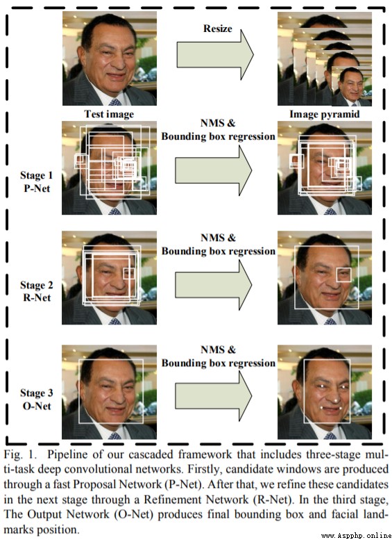
chart 2 MTCNN framework
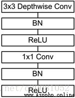
chart 3 MobileNet framework
_MobileNet_ The network structure is shown in the figure 3 Shown . The first is a 3x3 The standard convolution of , And then there's the pile depthwise separable convolution, And you can see some of them depthwise convolution Will pass strides=2 Conduct down sampling. Then use average pooling take feature become 1x1, Add the full connection layer according to the predicted category size , And finally a softmax layer .
Finally, the best value is batch_size=64,lr=0.0001,epochs=20, Other parameters are as follows , Train twice in a row , You can get the best results . Only the results under two parameters are shown here for comparison
# The size of a training set
batch_size = 64
# Compile model
model.compile(loss='binary_crossentropy', # Two class loss function
optimizer=Adam(lr=0.001), # Optimizer
metrics=['accuracy']) # Optimization objectives
# Training models
history = model.fit(train_generator,
epochs=20, # epochs: Integers , The total number of iterations of data .
# One epoch Number of steps included , Usually it should be equal to the number of samples in your dataset divided by the batch size .
steps_per_epoch=637 // batch_size,
validation_data=test_generator,
validation_steps=70 // batch_size,
initial_epoch=0, # Integers . Start training rounds ( It helps to get back to training ).
callbacks=[checkpoint_period, reduce_lr])
batch_size=48, lr=0.001,epochs=20, Test the model after training , The results are as follows :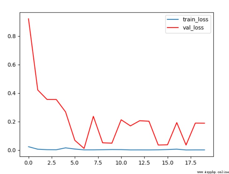
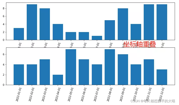
chart 4 Conditions 1 loss curve
from loss The curve shows , As the number of training iterations deepens , The loss on the verification set is gradually decreasing , Finally, it stabilized at 0.2 about ; And on the training set loss Always in 0 near .

chart 5 Conditions 1 acc curve
It can be seen from the accuracy change curve of verification set and test set , With the increase of training rounds , The accuracy of the validation set increases gradually , Finally, it stabilized at 96% about , The effect is good .
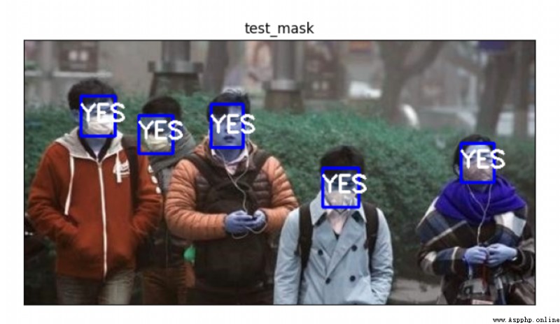
chart 6 Conditions 1 The test sample 1
Test with sample photos , Firstly, the face recognition part successfully recognized five faces , But the mask recognition part recognizes a person without a mask as a person with a mask , It shows that there is still room for progress , The actual error rate reached 20%.
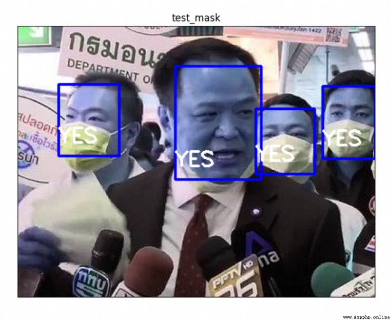
chart 7 Conditions 1 The test sample 2
The test result of another sample photo is that there is no problem in face recognition , Correctly recognized four faces , But also recognize a person without a mask as a person with a mask .

Subsequently, many experiments were carried out by adjusting various parameters and disturbing the picture order of the test set and training set , The final optimal state is as follows :
batch_size=64, lr=0.0001,epochs=20, Test the model after training , The results are as follows :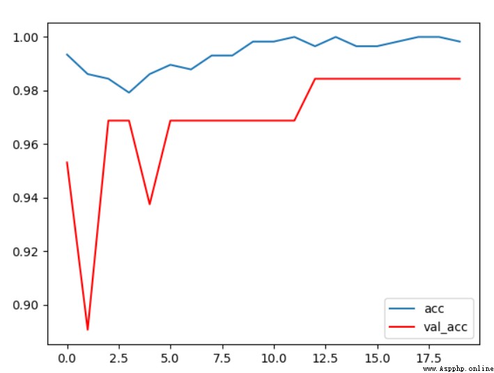
chart 8 Conditions 2 loss curve
By observing the accuracy curve, we can see , In this condition , The accuracy on the validation set is finally stable at 98% near , The effect is very good , It shows that some of the optimizations we have made have certain effects .
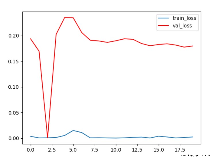
chart 9 Conditions 2 acc curve
Observe... Under this condition loss The curve shows the of the final validation set loss Stable at 0.2 about , Training set loss A very small , Basically close to 0
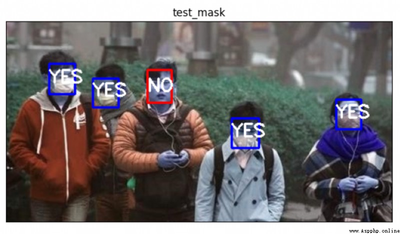
chart 10 Conditions 2 The test sample 1
Use two test samples to test the model , All inspection points in the first picture are correct , Five faces were correctly identified and the mask wearing test was correct , Recognition accuracy 100%.
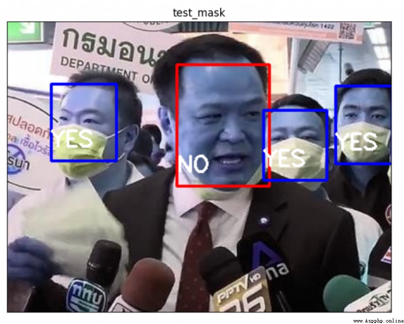
chart 11 Conditions 2 The test sample 2
Chapter 2 test examples , Correctly identified 4 Face and mask wearing test results are correct .
The test results of all test points on the two test samples are correct , Description under this parameter condition , The model recognition effect is good , It meets the requirements of mask wearing detection .

Use more test samples to find _MTCNN_ There is a problem that the face recognition part can not recognize the face correctly , Pass the test for many times , Revised mask_rec() The weight of the threshold function self.threshold, From the original self.threshold = [0.5,0.6,0.8] It is amended as follows self.threshold = [0.4,0.15,0.65]
Test with more self selected pictures locally , It is found that the accuracy of face recognition has improved . In terms of 2 When the training parameters remain unchanged , Use the same model for platform testing , give the result as follows :

Platform test scores have improved .
Continue to adjust mask_rec() The weight of the threshold function self.threshold, The weight of the threshold function is determined by system test feedback , Pass multiple tests , From the original self.threshold = [0.4,0.15,0.65] It is amended as follows self.threshold = [0.4,0.6,0.65]
Platform testing , give the result as follows :

Platform test scores have improved , achieve 95 branch .
In order to meet the conditions 4 The effect shown , A lot of attempts have been made on the value of threshold function , According to the feedback results of the submitted test , The final value is conditional 4 when , Can achieve the best . Because I don't know what the background test picture is and there is no feedback data , Therefore, the mask recognition model is still not improved by modifying the threshold function of face recognition again or modifying the parameters to train again .
Verification set accuracy
Test sample results
Platform performance
Conditions 1
96%
7/9
77.5
Conditions 2
98%
9/9
88.33333334
Conditions 3
98%
9/9
90
Conditions 4
98%
9/9
95
Finally, through continuous debugging and optimization of the algorithm , Got it 95 The platform score of points .
In this experiment, we mainly used _keras Methods training , Due to the initial use of these methods , Therefore, the process of early implementation is relatively difficult . At first I wanted to call GPU Resources to train , So I installed... For my computer tensorflow-gpu、CUDA And other supporting software and packages , Because the PC's graphics card version is older , So the installation process is also very tortuous . Fortunately, everything was finally installed , But because the video memory of the graphics card is relatively small , therefore bath_size The size can't go up , The maximum can only be given to 32, But it doesn't matter much . The process of adjusting parameters takes a lot of time , The optimization algorithm also takes a lot of time . Then the threshold function is modified , Although the process is very hard , But the final result is still very good , Finally, the whole reaches 95_ branch , On two given test samples, all test points are correct , Because I don't know what the five test photos of the platform are , So I don't know what went wrong , I hope the platform can feed back some modification suggestions later ~. In general, the harvest in the process is still great , Benefited greatly .
Training source code :
import warnings
# Ignore warning
warnings.filterwarnings('ignore')
import os
import matplotlib
import cv2 as cv
import numpy as np
import matplotlib.pyplot as plt
from tensorflow.keras.callbacks import ModelCheckpoint, ReduceLROnPlateau, EarlyStopping
from tensorflow.keras.applications.imagenet_utils import preprocess_input
from tensorflow.keras import backend as K
from tensorflow.keras.optimizers import Adam
K.image_data_format() == 'channels_last'
from keras_py.utils import get_random_data
from keras_py.face_rec import mask_rec
from keras_py.face_rec import face_rec
from keras_py.mobileNet import MobileNet
from tensorflow.keras.preprocessing.image import ImageDataGenerator
# Dataset path
basic_path = "./datasets/5f680a696ec9b83bb0037081-momodel/data/"
def letterbox_image(image, size): # Adjust the size of the picture , Return adjusted photos
new_image = cv.resize(image, size, interpolation=cv.INTER_AREA)
return new_image
read_img = cv.imread("test1.jpg")
print(" Adjust the size of the front picture :", read_img.shape)
read_img = letterbox_image(image=read_img, size=(50, 50))
print(" Adjust the size of the front picture :", read_img.shape)
def processing_data(data_path, height, width, batch_size=32, test_split=0.1): # Data processing ,batch_size The default size is 32
train_data = ImageDataGenerator(
# Multiply each pixel value of the picture by this zoom factor , Zoom the pixel value to 0 and 1 It is conducive to the convergence of the model
rescale=1. / 255,
# Floating point numbers , Shear strength ( Counterclockwise shear transformation angle )
shear_range=0.1,
# The amplitude of random scaling , If it is a floating point number , It's equivalent to [lower,upper] = [1 - zoom_range, 1+zoom_range]
zoom_range=0.1,
# Floating point numbers , A certain proportion of the width of the picture , The horizontal offset of the picture when the data is raised
width_shift_range=0.1,
# Floating point numbers , A certain proportion of the height of the picture , The vertical offset of the picture when the data is raised
height_shift_range=0.1,
# Boolean value , Do a random horizontal flip
horizontal_flip=True,
# Boolean value , Do a random vertical flip
vertical_flip=True,
# stay 0 and 1 Between the floating . The proportion of training data used as validation sets
validation_split=test_split
)
# Next, generate the test set , You can refer to the writing method of the training set
test_data = ImageDataGenerator(
rescale=1. / 255,
validation_split=test_split)
train_generator = train_data.flow_from_directory(
# A subdirectory is required under the provided path
data_path,
# Integer tuples (height, width), Default :(256, 256). All images will be resized .
target_size=(height, width),
# The size of a batch of data
batch_size=batch_size,
# "categorical", "binary", "sparse", "input" or None One of .
# Default :"categorical", return one-hot Code tags .
class_mode='categorical',
# Data subsets ("training" or "validation")
subset='training',
seed=0)
test_generator = test_data.flow_from_directory(
data_path,
target_size=(height, width),
batch_size=batch_size,
class_mode='categorical',
subset='validation',
seed=0)
return train_generator, test_generator
# Data path
data_path = basic_path + 'image'
# The number of rows and columns of image data
height, width = 160, 160
# Obtain training data and validation data set
train_generator, test_generator = processing_data(data_path, height, width)
# Passing attribute class_indices The corresponding Dictionary of folder name and class sequence number can be obtained .
labels = train_generator.class_indices
print(labels)
# Convert to the dictionary corresponding to the sequence number of the class and the folder name
labels = dict((v, k) for k, v in labels.items())
print(labels)
pnet_path = "./datasets/5f680a696ec9b83bb0037081-momodel/data/keras_model_data/pnet.h5"
rnet_path = "./datasets/5f680a696ec9b83bb0037081-momodel/data/keras_model_data/rnet.h5"
onet_path = "./datasets/5f680a696ec9b83bb0037081-momodel/data/keras_model_data/onet.h5"
# load MobileNet Pre training model weight
weights_path = basic_path + 'keras_model_data/mobilenet_1_0_224_tf_no_top.h5'
# The number of rows and columns of image data
height, width = 160, 160
model = MobileNet(input_shape=[height,width,3],classes=2)
model.load_weights(weights_path,by_name=True)
print(' Loading complete ...')
def save_model(model, checkpoint_save_path, model_dir): # Save the model
if os.path.exists(checkpoint_save_path):
print(" Model loading ")
model.load_weights(checkpoint_save_path)
print(" The model is loaded ")
checkpoint_period = ModelCheckpoint(
# Model storage path
model_dir + 'ep{epoch:03d}-loss{loss:.3f}-val_loss{val_loss:.3f}.h5',
# Test indicators
monitor='val_acc',
# ‘auto’,‘min’,‘max’ Choose from
mode='max',
# Whether only model weights are stored
save_weights_only=False,
# Whether to save only the optimal model
save_best_only=True,
# The number of rounds tested is every 2 round
period=2
)
return checkpoint_period
checkpoint_save_path = "./results/last_one88.h5"
model_dir = "./results/"
checkpoint_period = save_model(model, checkpoint_save_path, model_dir)
# The way the learning rate decreases ,acc If you don't drop three times, you'll drop your learning rate and continue training
reduce_lr = ReduceLROnPlateau(
monitor='accuracy', # Test indicators
factor=0.5, # When acc The proportion of reducing the learning rate when it does not decline
patience=3, # The number of inspection rounds is every three rounds
verbose=2 # Information display mode
)
early_stopping = EarlyStopping(
monitor='val_accuracy', # Test indicators
min_delta=0.0001, # Increasing or decreasing threshold
patience=3, # Number and frequency of rounds tested
verbose=1 # Mode of information display
)
# The size of a training set
batch_size = 64
# Picture data path
data_path = basic_path + 'image'
# The image processing
train_generator, test_generator = processing_data(data_path, height=160, width=160, batch_size=batch_size, test_split=0.1)
# Compile model
model.compile(loss='binary_crossentropy', # Two class loss function
optimizer=Adam(lr=0.001), # Optimizer
metrics=['accuracy']) # Optimization objectives
# Training models
history = model.fit(train_generator,
epochs=20, # epochs: Integers , The total number of iterations of data .
# One epoch Number of steps included , Usually it should be equal to the number of samples in your dataset divided by the batch size .
steps_per_epoch=637 // batch_size,
validation_data=test_generator,
validation_steps=70 // batch_size,
initial_epoch=0, # Integers . Start training rounds ( It helps to get back to training ).
callbacks=[checkpoint_period, reduce_lr])
# Save the model
model.save_weights(model_dir + 'temp.h5')
plt.plot(history.history['loss'],label = 'train_loss')
plt.plot(history.history['val_loss'],'r',label = 'val_loss')
plt.legend()
plt.show()
plt.plot(history.history['accuracy'],label = 'acc')
plt.plot(history.history['val_accuracy'],'r',label = 'val_acc')
plt.legend()
plt.show()