您现在的位置：程式師世界 >> 編程語言 > >> 更多編程語言 >> Python

Basic concepts of SVM and python implementation code

編輯：Python

SVM（support vector machine） Support vector machine ：

Be careful ： This article is not going to mention the process of mathematical proof , One is that there is a very good article that explains it very well ： General introduction to support vector machines （ understand SVM Three levels of state ） , On the other hand, I am just a programmer , Not a math guy （ It's mainly because math is not good .）, The main purpose is to SVM In the most accessible , Explain clearly in a simple and crude way .

Linear classification ：

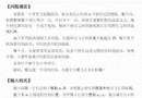
Let's start with linearly separable data , If the data to be classified are linearly separable , Then you just need a straight line f(x)=wx+b You can separate , Like this ：

This method is called ： Linear classifier , The learning goal of a linear classifier is to n Find a hyperplane in the data space of dimension （hyper plane）. in other words , Data is not always two-dimensional , such as , A three-dimensional hyperplane is a face . But there's a problem ：

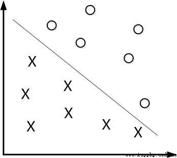
These two hyperplanes , Can classify the data , From this, we can deduce , In fact, there can be countless hyperplanes that can divide the data , But which is the best ？

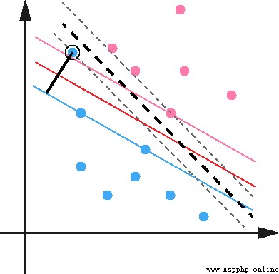
Maximum interval classifier Maximum Margin Classifier：

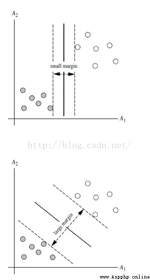
abbreviation MMH, Classify a data point , When the hyperplane is away from the data point “ interval ” The bigger it is , Certainty of classification （confidence） The greater the . therefore , In order to make the classification as sure as possible , We need to maximize this by choosing a hyperplane “ interval ” value . This interval is shown below Gap Half of .

The point used to generate the support vector , Pictured above XO, Called support vector points , therefore SVM There is an advantage , Even if there is a lot of data , But support vector points are fixed , So even if you train a lot of data again , This hyperplane may not change .

Nonlinear classification ：

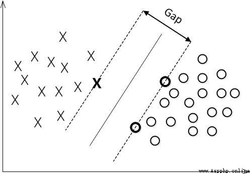
Data can't be linear in most cases , How to segment non-linear data ？

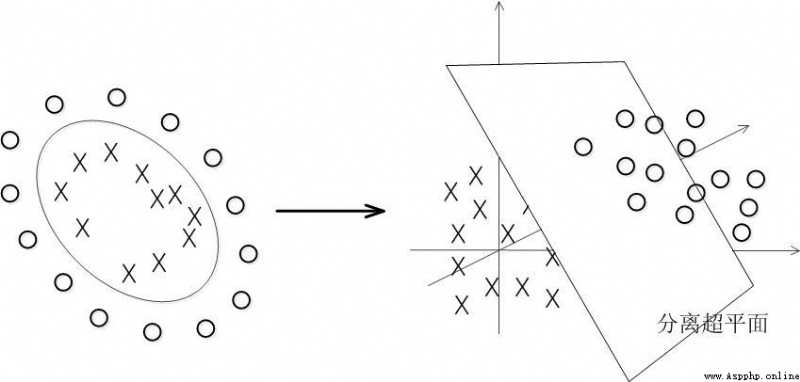
The solution is to put the data on a high dimension and then split it , Here's the picture ：

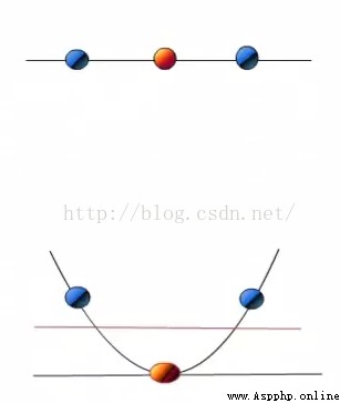
When f(x)=x when , This set of data is a straight line , The upper half , But when I turn this set of data into f(x)=x^2 when , This set of data becomes the lower part , It can be divided by the red line .

for instance , I have a set of three-dimensional data here X=（x1,x2,x3）, Linear indivisible , So I need to convert it to six-dimensional space . So we can assume that the six dimensions are ：x1,x2,x3,x1^2,x1*x2,x1*x3, Of course, it can continue to unfold , But in six dimensions, that's enough .

New decision hyperplane ：d(Z)=WZ+b, figure out W and b Then bring it into the equation , Therefore, the hyperplane of this set of data should be ：d(Z)=w1x1+w2x2+w3x3+w4*x1^2+w5x1x2+w6x1x3+b But there is a new problem , The conversion of high latitude is generally based on inner product （dot product） In the way of , But the algorithm complexity of inner product is very large .

Kernel function Kernel：

We often encounter examples of linear indivisibility , here , Our common practice is to map sample features to high-dimensional space . But further , If we encounter linear indivisible examples , All map to high dimensional space , So the dimension size is going to be terrible , And the inner product method is too complicated . here , The kernel function is on the stage , The value of kernel function is that although it is also about feature transformation from low dimension to high dimension , But the kernel function must be calculated in the low dimension in advance , And the classification effect in essence is shown in the high dimension , As mentioned above, the complex computation directly in high-dimensional space is avoided .

Several common kernel functions ：

h Degree polynomial kernel function （Polynomial Kernel of Degree h）

Gaussian radial basis and function （Gaussian radial basis function Kernel）

S Type kernel function （Sigmoid function Kernel）

Image classification , Gaussian radial basis functions and , Because the classification is smoother , Text does not apply to Gaussian radial basis functions . There is no standard answer , You can try various kernel functions , Judge according to the accuracy .

Relax variables ：

The data itself may have noise , It will make the originally linearly separable data need to be mapped to high dimensions . For this kind of data point far away from the normal position , We call it outlier , In our original SVM In the model ,outlier The existence of the can have a big impact , Because the hyperplane itself is just a few support vector Composed of , If these support vector There's... In it outlier Words , The impact is great .

Thus eliminate outlier spot , It can improve the accuracy of the model and avoid Overfitting The way .

Solve the problem of multi classification ：

classical SVM Only two kinds of classification algorithms are given , In reality, data may need to solve the problem of multi class classification . So it can be run many times SVM, Generate multiple hyperplanes , If classification is required 1-10 Products , First find 1 and 2-10 The hyperplane of , Search again 2 and 1,3-10 The hyperplane of , And so on , Finally, when you need to test data , According to the corresponding distance or distribution .

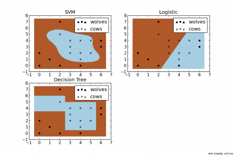
SVM Compared with other machine learning algorithms ( chart )：