Logistic regression algorithm is a widely used classification algorithm , Through the positive and negative samples in the training data , Learn the hypothetical function between sample characteristics and sample labels . Logistic regression assumes that the dependent variable y Obey the Bernoulli distribution , Linear regression assumes that the dependent variable y Obey Gauss distribution . So it has a lot in common with linear regression , Remove Sigmoid Mapping function , The logistic regression algorithm is a linear regression .
advantage :
(1) It is suitable for the problem of dichotomy , No need to scale input features ;
(2) The memory resource is small , Because you only need to store the eigenvalues of each dimension ;
(3) Fast training ;
shortcoming :
(1) We cannot use logistic regression to solve nonlinear problems , because Logistic The decision surface is linear ;
(2) The accuracy is not very high , Because the form is very simple ( It's very similar to a linear model ), It's hard to fit the real distribution of the data ;
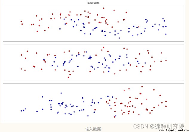
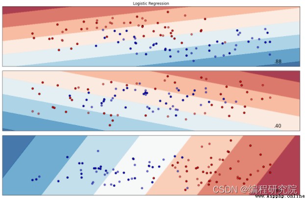
Python Code implementation
# iterate over datasets
for ds_cnt, ds in enumerate(datasets):
# iterate over classifiers
for name, clf in zip(names, classifiers):
ax = plt.subplot(len(datasets), len(classifiers) + 1, i)
clf.fit(X_train, y_train)
score = clf.score(X_test, y_test)
# Plot the decision boundary. For that, we will assign a color to each
# point in the mesh [x_min, x_max]x[y_min, y_max].
if hasattr(clf, "decision_function"):
Z = clf.decision_function(np.c_[xx.ravel(), yy.ravel()])
else:
Z = clf.predict_proba(np.c_[xx.ravel(), yy.ravel()])[:, 1]
# Put the result into a color plot
Z = Z.reshape(xx.shape)
ax.contourf(xx, yy, Z, cmap=cm, alpha=.8)
# Plot also the training points
ax.scatter(X_train[:, 0], X_train[:, 1], c=y_train, cmap=cm_bright,
edgecolors='k')
# and testing points
ax.scatter(X_test[:, 0], X_test[:, 1], c=y_test, cmap=cm_bright,
edgecolors='k', alpha=0.6)
ax.set_xlim(xx.min(), xx.max())
ax.set_ylim(yy.min(), yy.max())
ax.set_xticks(())
ax.set_yticks(())
if ds_cnt == 0:
ax.set_title(name)
ax.text(xx.max() - .3, yy.min() + .3, ('%.2f' % score).lstrip('0'),
size=15, horizontalalignment='right')
i += 1
plt.tight_layout()
plt.show()
The output results are as follows :
Friends who want complete code , can toutiao Search on “ Programming workshop ” After attention s Believe in me , reply “ Algorithm notes 11“ Free access