Introduce dependencies
Algorithm dependent
get data
Generate df
To be ranked high
Add column
Missing value processing
Hot coding alone
Replacement value
Delete column
Data filtering
Difference calculation
Data modification
Time format conversion
Set index columns
Broken line diagram
Scatter plot
Histogram
Heat map
66 The most commonly used pandas Data analysis function
Import data from a variety of sources and formats
Derived data
Create test object
see 、 Check the data
Data selection
Data cleaning
Screening , Sort and group by
Data merging
Data statistics
16 A function , For data cleaning
1.cat function
2.contains
3.startswith/endswith
4.count
5.get
6.len
7.upper/lower
8.pad+side Parameters /center
9.repeat
10.slice_replace
11.replace
12.replace
13.split Method +expand Parameters
14.strip/rstrip/lstrip
15.findall
16.extract/extractall
Introduce dependencies# The import module import pymysqlimport pandas as pdimport numpy as npimport time# database from sqlalchemy import create_engine# visualization import matplotlib.pyplot as plt# If your equipment is equipped with Retina Of the screen mac, Can be in jupyter notebook in , Use the following line of code to effectively improve the image quality %config InlineBackend.figure_format = 'retina'# solve plt The problem of Chinese display mymacplt.rcParams['font.sans-serif'] = ['Arial Unicode MS']# Set display Chinese You need to install fonts first aistudioplt.rcParams['font.sans-serif'] = ['SimHei'] # Specify default font plt.rcParams['axes.unicode_minus'] = False # Used to display negative sign normally import seaborn as sns# notebook Rendering pictures %matplotlib inlineimport pyecharts# Ignore version issues import warningswarnings.filterwarnings("ignore") # Download Chinese Fonts !wget https://mydueros.cdn.bcebos.com/font/simhei.ttf # Copy the font file to matplotlib' The font path !cp simhei.ttf /opt/conda/envs/python35-paddle120-env/Lib/python3,7/site-packages/matplotib/mpl-data/fonts.# Generally, you only need to copy the font file to the system font field and record it , But in studio There is no write permission on this path , So this method cannot be used # !cp simhei. ttf /usr/share/fonts/# Create system font file path !mkdir .fonts# Copy files to this path !cp simhei.ttf .fonts/!rm -rf .cache/matplotlib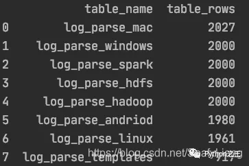
# Data normalization from sklearn.preprocessing import MinMaxScaler# kmeans clustering from sklearn.cluster import KMeans# DBSCAN clustering from sklearn.cluster import DBSCAN# Linear regression algorithm from sklearn.linear_model import LinearRegression# Logic regression algorithm from sklearn.linear_model import LogisticRegression# Gauss bayes from sklearn.naive_bayes import GaussianNB# Divide training / Test set from sklearn.model_selection import train_test_split# Accuracy report from sklearn import metrics# Matrix report and mean square error from sklearn.metrics import classification_report, mean_squared_error get data from sqlalchemy import create_engineengine = create_engine('mysql+pymysql://root:[email protected]:3306/ry?charset=utf8')# Query the related table name and row number after insertion result_query_sql = "use information_schema;"engine.execute(result_query_sql)result_query_sql = "SELECT table_name,table_rows FROM tables WHERE TABLE_NAME LIKE 'log%%' order by table_rows desc;"df_result = pd.read_sql(result_query_sql, engine)
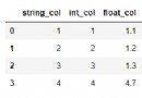
# list turn dfdf_result = pd.DataFrame(pred,columns=['pred'])df_result['actual'] = test_targetdf_result# df Take a seed dfdf_new = df_old[['col1','col2']]# dict Generate dfdf_test = pd.DataFrame({<!-- -->'A':[0.587221, 0.135673, 0.135673, 0.135673, 0.135673], 'B':['a', 'b', 'c', 'd', 'e'], 'C':[1, 2, 3, 4, 5]})# Specifies the column name data = pd.DataFrame(dataset.data, columns=dataset.feature_names)# Use numpy Generate 20 A specified distribution ( Such as standard normal distribution ) Number of numbers tem = np.random.normal(0, 1, 20)df3 = pd.DataFrame(tem)# Generate a and df Random numbers of the same length dataframedf1 = pd.DataFrame(pd.Series(np.random.randint(1, 10, 135))) To be ranked high # To be ranked high data_scaled = data_scaled.rename(columns={<!-- -->' Body oil level ': 'OILLV'}) Add column # df2dfdf_jj2yyb['r_time'] = pd.to_datetime(df_jj2yyb['cTime'])# Add a new column based on salary Divide the data into 3 Group bins = [0,5000, 20000, 50000]group_names = [' low ', ' in ', ' high ']df['categories'] = pd.cut(df['salary'], bins, labels=group_names) Missing value processing # Check the data for any missing values df.isnull().values.any()# Check the missing values of each column df.isnull().sum()# Extract a row with a null value in a column df[df[' date '].isnull()]# Output the specific number of missing rows in each column for i in df.columns: if df[i].count() != len(df): row = df[i][df[i].isnull().values].index.tolist() print(' Name :"{}", The first {} Line position has missing value '.format(i,row))# Mode filling heart_df['Thal'].fillna(heart_df['Thal'].mode(dropna=True)[0], inplace=True)# The empty values of the continuous value column are filled with the average value dfcolumns = heart_df_encoded.columns.values.tolist()for item in dfcolumns: if heart_df_encoded[item].dtype == 'float': heart_df_encoded[item].fillna(heart_df_encoded[item].median(), inplace=True) Hot coding alone df_encoded = pd.get_dummies(df_data) Replacement value # Replace by column value num_encode = {<!-- --> 'AHD': {<!-- -->'No':0, "Yes":1},}heart_df.replace(num_encode,inplace=True) Delete column df_jj2.drop(['coll_time', 'polar', 'conn_type', 'phase', 'id', 'Unnamed: 0'],axis=1,inplace=True) Data filtering # Take the first place 33 Row data df.iloc[32]# A column with xxx Start of string df_jj2 = df_512.loc[df_512["transformer"].str.startswith('JJ2')]df_jj2yya = df_jj2.loc[df_jj2[" Transformer No "]=='JJ2YYA']# Extract numbers that do not appear in the second column in the first column df['col1'][~df['col1'].isin(df['col2'])]# Find row numbers with equal values in two columns np.where(df.secondType == df.thirdType)# Include string results = df['grammer'].str.contains("Python")# Extract column names df.columns# View the unique value of a column ( species )df['education'].nunique()# Delete duplicate data df.drop_duplicates(inplace=True)# A value is equal to a column df[df.col_name==0.587221]# df.col_name==0.587221 The return value of each row judgment result (True/False)# View the unique value and count of a column df_jj2[" Transformer No "].value_counts()# Time period filtering df_jj2yyb_0501_0701 = df_jj2yyb[(df_jj2yyb['r_time'] >=pd.to_datetime('20200501')) & (df_jj2yyb['r_time'] <= pd.to_datetime('20200701'))]# Numerical filtering df[(df['popularity'] > 3) & (df['popularity'] < 7)]# A column of string is intercepted df['Time'].str[0:8]# Random selection num That's ok ins_1 = df.sample(n=num)# Data De duplication df.drop_duplicates(['grammer'])# Sort by a column ( Descending )df.sort_values("popularity",inplace=True, ascending=False)# Take the maximum value of a row df[df['popularity'] == df['popularity'].max()]# Take the maximum of a column num That's ok df.nlargest(num,'col_name')# Maximum num Draw a horizontal column df.nlargest(10).plot(kind='barh')
# axis=0 or index Move up and down , periods Indicates the number of moves , For timing, move down , Move up when negative .print(df.diff( periods=1, axis=‘index‘))print(df.diff( periods=-1, axis=0))# axis=1 or columns Move left and right ,periods Indicates the number of moves , Shift right for timing , Move left when negative .print(df.diff( periods=1, axis=‘columns‘))print(df.diff( periods=-1, axis=1))# Rate of change calculation data[' Closing price ( element )'].pct_change()# With 5 Data as a data sliding window , In this 5 Average on data df[' Closing price ( element )'].rolling(5).mean() Data modification # Delete last line df = df.drop(labels=df.shape[0]-1)# Add a row of data ['Perl',6.6]row = {<!-- -->'grammer':'Perl','popularity':6.6}df = df.append(row,ignore_index=True)# A column of decimals to percentages df.style.format({<!-- -->'data': '{0:.2%}'.format})# Reverse transfer df.iloc[::-1, :]# Make a PivotTable with two columns pd.pivot_table(df,values=["salary","score"],index="positionId")# Calculate the two columns at the same time df[["salary","score"]].agg([np.sum,np.mean,np.min])# Perform different calculations for different columns df.agg({<!-- -->"salary":np.sum,"score":np.mean}) Time format conversion # Timestamp to time string df_jj2['cTime'] =df_jj2['coll_time'].apply(lambda x: time.strftime("%Y-%m-%d %H:%M:%S", time.localtime(x)))# Time string to time format df_jj2yyb['r_time'] = pd.to_datetime(df_jj2yyb['cTime'])# Time format to timestamp dtime = pd.to_datetime(df_jj2yyb['r_time'])v = (dtime.values - np.datetime64('1970-01-01T08:00:00Z')) / np.timedelta64(1, 'ms')df_jj2yyb['timestamp'] = v Set index columns df_jj2yyb_small_noise = df_jj2yyb_small_noise.set_index('timestamp') Broken line diagram fig, ax = plt.subplots()df.plot(legend=True, ax=ax)plt.legend(loc=1)plt.show()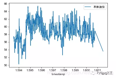
plt.figure(figsize=(20, 6))plt.plot(max_iter_list, accuracy, color='red', marker='o', markersize=10)plt.title('Accuracy Vs max_iter Value')plt.xlabel('max_iter Value')plt.ylabel('Accuracy')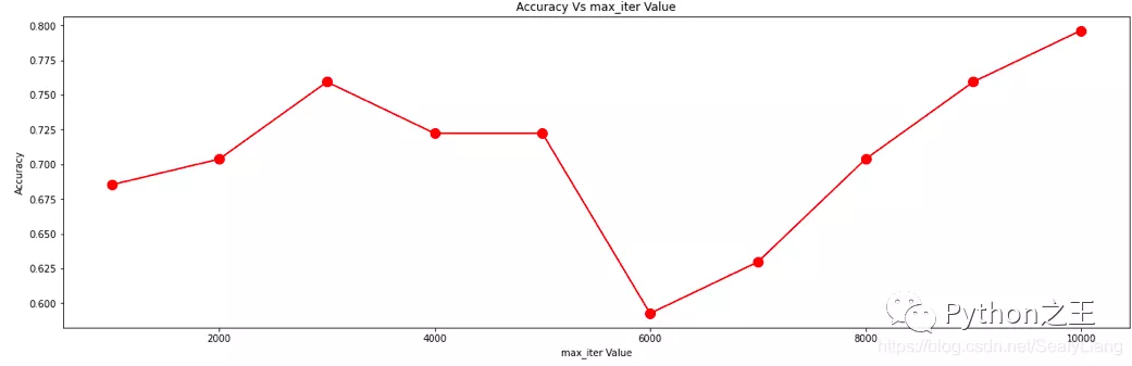
plt.scatter(df[:, 0], df[:, 1], c="red", marker='o', label='lable0') plt.xlabel('x') plt.ylabel('y') plt.legend(loc=2) plt.show() 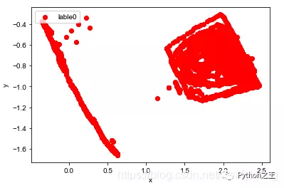
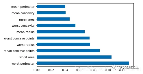
df = pd.Series(tree.feature_importances_, index=data.columns)# Take the maximum of a column Num Draw a horizontal column in a row df.nlargest(10).plot(kind='barh')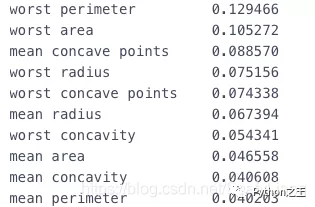
df_corr = combine.corr()plt.figure(figsize=(20,20))g=sns.heatmap(df_corr,annot=True,cmap="RdYlGn")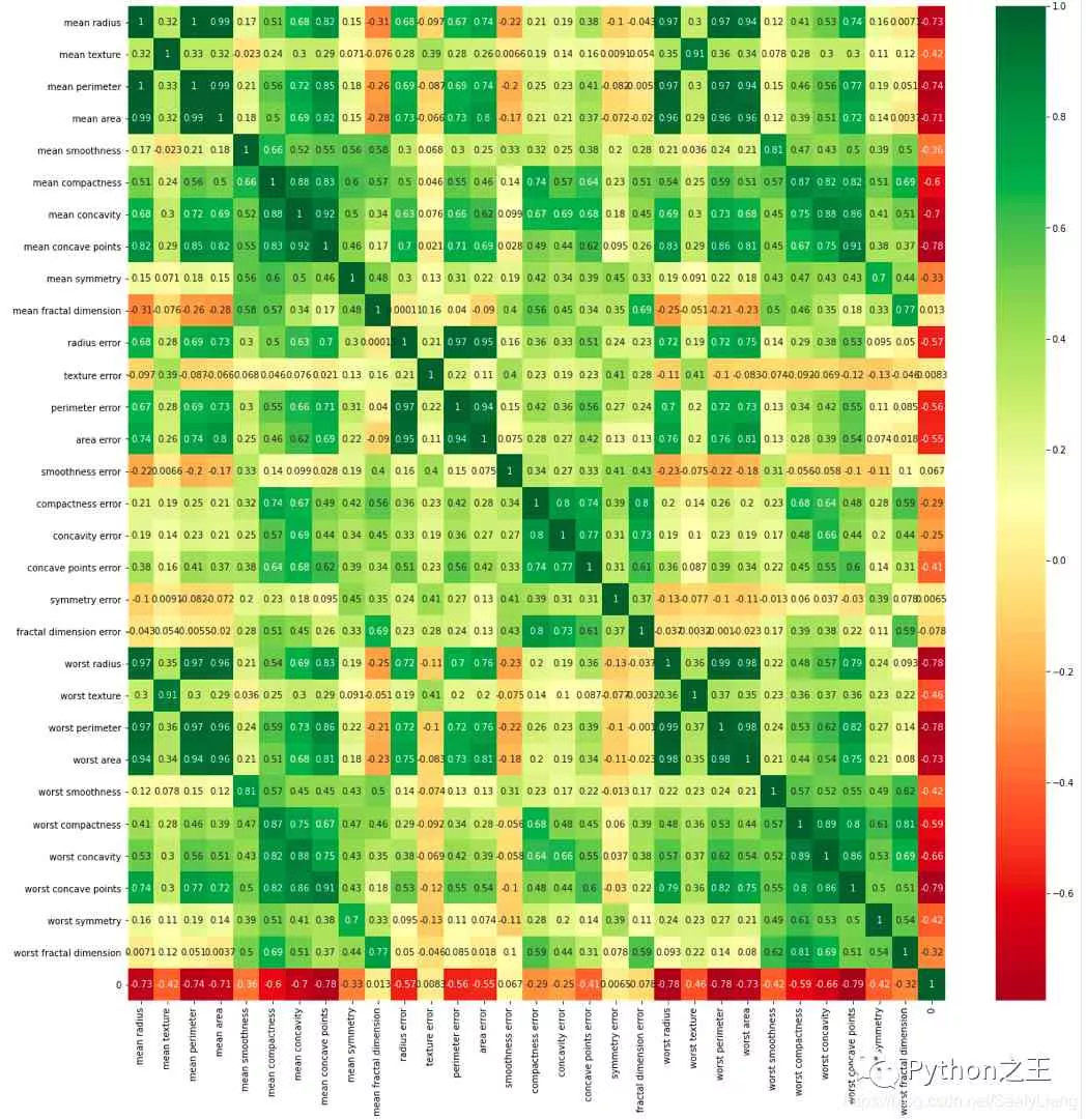
df # whatever pandas DataFrame object s # whatever pandas series object Import data from a variety of sources and formats pd.read_csv(filename) # from CSV file pd.read_table(filename) # From delimited text files ( for example CSV) in pd.read_excel(filename) # from Excel file pd.read_sql(query, connection_object) # from SQL surface / Read from the database pd.read_json(json_string) # from JSON Format string ,URL Or file .pd.read_html(url) # analysis html URL, String or file , And extract the table into the data frame list pd.read_clipboard() # Get the contents of the clipboard and pass it to read_table() pd.DataFrame(dict) # From the dictionary , The key of the column name , The value of the data in the list Derived data df.to_csv(filename) # write in CSV file df.to_excel(filename) # write in Excel file df.to_sql(table_name, connection_object) # write in SQL surface df.to_json(filename) # With JSON Format write file Create test object pd.DataFrame(np.random.rand(20,5)) # 5 Column 20 Row random floating point number pd.Series(my_list) # Create a sequence from an iterative sequence my_list df.index = pd.date_range('1900/1/30', periods=df.shape[0]) # Add date index see 、 Check the data df.head(n) # DataFrame Before n That's ok df.tail(n) # DataFrame Last n That's ok df.shape # Number of rows and columns df.info() # Indexes , Data types and memory information df.describe() # Summary statistics for numeric columns s.value_counts(dropna=False) # View unique values and counts df.apply(pd.Series.value_counts) # Unique values and counts for all columns Data selection Use these commands to select a specific subset of the data .df[col] # Return with label col The column of df[[col1, col2]] # Returns the column as a new DataFrame s.iloc[0] # Select by location s.loc['index_one'] # Select by index df.iloc[0,:] # first line df.iloc[0,0] # The first element of the first column Data cleaning df.columns = ['a','b','c'] # To be ranked high pd.isnull() # Null check , return Boolean Arrray pd.notnull() # And pd.isnull() contrary df.dropna() # Delete all rows with null values df.dropna(axis=1) # Delete all columns with null values df.dropna(axis=1,thresh=n) # Delete all with less than n A non null Row of values df.fillna(x) # Replace all null values with x s.fillna(s.mean()) # Replace all null values with the mean ( The mean can be replaced by almost all functions in the statistics module ) s.astype(float) # Convert the data type of the series to float s.replace(1,'one') # 1 use 'one' s.replace([1,3],['one','three']) # Replace all values equal to Replace with all 1 'one' , and 3 use 'three' df.rename(columns=lambda x: x + 1) # Renaming Columns df.rename(columns={<!-- -->'old_name': 'new_ name'})# Selective renaming df.set_index('column_one') # Change index df.rename(index=lambda x: x + 1) # Large scale index renaming Screening , Sort and group by df[df[col] > 0.5] # Column col Greater than 0.5 df[(df[col] > 0.5) & (df[col] < 0.7)] # Less than 0.7 Greater than 0.5 The line of df.sort_values(col1) # Press col1 Sort values in ascending order df.sort_values(col2,ascending=False) # Press col2 Values are sorted in descending order Sort df.sort_values([col1,col2],ascending=[True,False]) # Press col1 Ascending sort , then col2 Sort in descending order df.groupby(col) # Return from a column GROUPBY object df.groupby([col1,col2]) # Returns from multiple columns groupby object df.groupby(col1)[col2] # Returns the average of the values in col2, Group by value in col1 ( The average value can be replaced by almost all functions in the statistics module ) df.pivot_table(index=col1,values=[col2,col3],aggfunc=mean) # Create a PivotTable group through col1 , And calculate the average col2 and col3 df.groupby(col1).agg(np.mean) # Find each unique... In all columns col1 Group average df.apply(np.mean) #np.mean() Apply this function on each column df.apply(np.max,axis=1) # np.max() Apply functions on each line Data merging df1.append(df2) # take df2 add to df1 At the end of ( Each column should be the same ) pd.concat([df1, df2],axis=1) # take df1 Add columns to df2 At the end of ( Lines should be the same ) df1.join(df2,on=col1,how='inner') # SQL The style will be column df1 And df2 The column in which the row is located col Join columns with the same value .'how' It could be a 'left', 'right', 'outer', 'inner' Data statistics df.describe() # Summary statistics for numeric columns df.mean() # Returns all columns of the mean df.corr() # return DataFrame Correlation between columns in df.count() # Returns the number in each data frame column with a non null value df.max() # Returns the highest value in each column df.min() # Returns the minimum value in each column df.median() # Returns the median of each column df.std() # Returns the standard deviation of each column 16 A function , For data cleaning # Import dataset import pandas as pddf ={<!-- -->' full name ':[' Schoolmate Huang ',' Huang Zhizun ',' Huanglaoxie ',' Chen Dami ',' Sun shangxiang '], ' English name ':['Huang tong_xue','huang zhi_zun','Huang Lao_xie','Chen Da_mei','sun shang_xiang'], ' Gender ':[' male ','women','men',' Woman ',' male '], ' Id card ':['463895200003128433','429475199912122345','420934199110102311','431085200005230122','420953199509082345'], ' height ':['mid:175_good','low:165_bad','low:159_bad','high:180_verygood','low:172_bad'], ' Home address ':[' Guangshui, Hubei Province ',' Xinyang, Henan ',' Guangxi Guilin ',' Xiaogan, Hubei ',' Guangdong guangzhou '], ' Phone number ':['13434813546','19748672895','16728613064','14561586431','19384683910'], ' income ':['1.1 ten thousand ','8.5 thousand ','0.9 ten thousand ','6.5 thousand ','2.0 ten thousand ']}df = pd.DataFrame(df)df1.cat function For string splicing
df[" full name "].str.cat(df[" Home address "],sep='-'*3)2.containsDetermine whether a string contains a given character
df[" Home address "].str.contains(" wide ")3.startswith/endswithDetermine whether a string is represented by … start / ending
# The first line “ Huang Wei ” It starts with a space df[" full name "].str.startswith(" yellow ") df[" English name "].str.endswith("e")4.countCalculates the number of occurrences of a given character in a string
df[" Phone number "].str.count("3")5.getGets the string at the specified location
df[" full name "].str.get(-1)df[" height "].str.split(":")df[" height "].str.split(":").str.get(0)6.lenCalculate string length
df[" Gender "].str.len()7.upper/lowerEnglish case conversion
df[" English name "].str.upper()df[" English name "].str.lower()8.pad+side Parameters /centerTo the left of the string 、 Add the given character to the right or left
df[" Home address "].str.pad(10,fillchar="*") # amount to ljust()df[" Home address "].str.pad(10,side="right",fillchar="*") # amount to rjust()df[" Home address "].str.center(10,fillchar="*")9.repeatRepeat string several times
df[" Gender "].str.repeat(3)10.slice_replaceUse the given string , Replace the character at the specified position
df[" Phone number "].str.slice_replace(4,8,"*"*4)11.replaceThe character at the specified position , Replace with the given string
df[" height "].str.replace(":","-")12.replaceThe character at the specified position , Replace with the given string ( Accept regular expressions )
replace Pass in regular expression , It's easy to use ;- Don't worry about whether the following case is useful , You just need to know , How easy it is to use regular data cleaning ;
df[" income "].str.replace("\d+\.\d+"," Regular ")13.split Method +expand Parameters collocation join Methods are powerful
# Common usage df[" height "].str.split(":")# split Method , collocation expand Parameters df[[" Height description ","final height "]] = df[" height "].str.split(":",expand=True)df# split Method collocation join Method df[" height "].str.split(":").str.join("?"*5)14.strip/rstrip/lstripRemove blanks 、 A newline
df[" full name "].str.len()df[" full name "] = df[" full name "].str.strip()df[" full name "].str.len()15.findallUsing regular expressions , To match... In a string , Returns a list of search results
findall Using regular expressions , Do data cleaning , It's really fragrant !
df[" height "]df[" height "].str.findall("[a-zA-Z]+")16.extract/extractallAccept regular expressions , Extract the matching string ( Be sure to put parentheses )
df[" height "].str.extract("([a-zA-Z]+)")# extractall Extract the composite index df[" height "].str.extractall("([a-zA-Z]+)")# extract collocation expand Parameters df[" height "].str.extract("([a-zA-Z]+).*?([a-zA-Z]+)",expand=TrueThat's all Python Pandas Details of high-frequency operation of data processing , More about Python Pandas For data processing information, please pay attention to other relevant articles on the software development network !