introduction
scikit-image Digital image processing
Image information
skimage Sub modules of the package
Read the picture from the outside and display
The program comes with pictures
Save the picture
Image pixel access and cropping
color Modular rgb2gray() function
result
Image data type and color space conversion
1、unit8 turn float
2、float turn uint8
Other conversions
Drawing of image
Other methods of drawing and displaying
Batch processing of images
Image deformation and scaling
1、 Change the picture size resize
2、 To scale rescale
3、 rotate rotate
4、 Image pyramid
Contrast and brightness adjustment
1、gamma adjustment
2、log Logarithmic adjustment
3、 Judge whether the image contrast is low
4、 Adjust the intensity
Histogram and equalization
2、 Draw histogram
3、 Color picture three channel histogram
4、 Histogram equalization
CLAHE
introduction be based on python Script language development of digital image processing package , such as PIL,Pillow, opencv, scikit-image etc. .
PIL and Pillow Only the most basic digital image processing , Limited function ;
opencv It's actually a c++ library , It just provides python Interface , The update speed is very slow .scikit-image Is based on scipy An image processing package , It takes pictures as numpy Array processing , Coincide with matlab equally , therefore , We finally choose scikit-image Digital image processing .
scikit-image Digital image processingImage What I read is PIL The type of , and skimage.io The data read out is numpy Format
import Image as imgimport osfrom matplotlib import pyplot as plotfrom skimage import io,transform#Image and skimage Read pictures img_file1 = img.open('./CXR_png/MCUCXR_0042_0.png')img_file2 = io.imread('./CXR_png/MCUCXR_0042_0.png')The output shows Img The size of the reading picture is the size of the picture (width, height); and skimage Yes. (height,width, channel), [ That's why caffe When testing separately, you need to set... In the code :transformer.set_transpose('data',(2,0,1)), because caffe The data format of the picture that can be processed is (channel,height,width), So you have to convert the data ]
# The size of the data after reading the picture :print "the picture's size: ", img_file1.sizeprint "the picture's shape: ", img_file2.shapethe picture's size: (4892, 4020)the picture's shape: (4020, 4892)# Get pixel :print(img_file1.getpixel((500,1000)), img_file2[500][1000])print(img_file1.getpixel((500,1000)), img_file2[1000][500])print(img_file1.getpixel((1000,500)), img_file2[500][1000])(0, 139)
(0, 0)
(139, 139)
Img Read out the picture to get a certain pixel getpixel((w,h)) You can directly return the pixel values of the three channels at this point
skimage The pictures can be read directly img_file2[0][0] get , But remember the format , Not what you think (channel,height,width)
If we want to know something skimage Image information
from skimage import io, dataimg = data.chelsea()io.imshow(img)print(type(img)) # Display type print(img.shape) # Display size print(img.shape[0]) # Picture height print(img.shape[1]) # Image width print(img.shape[2]) # Number of picture channels print(img.size) # Displays the total number of pixels print(img.max()) # Maximum pixel value print(img.min()) # Minimum pixel value print(img.mean()) # Pixel average print(img[0][0])# The pixel value of the image PIL image Check the picture information , The following methods can be used
print type(img)print img.size # The size of the picture print img.mode # The pattern of the picture print img.format # The format of the picture print(img.getpixel((0,0)))# Get pixel :#img Read out the picture to get a certain pixel getpixel((w,h)) You can directly return the pixel values of the three channels at this point # Obtain the gray value range of the image width = img.size[0]height = img.size[1]# Output the pixel value of the picture count = 0 for i in range(0, width): for j in range(0, height): if img.getpixel((i, j))>=0 and img.getpixel((i, j))<=255: count +=1print countprint(height*width)skimage Provides io modular , seeing the name of a thing one thinks of its function , This module is used for image input and output operation . To facilitate practice , There is also a data modular , Some sample pictures are nested inside , We can use it directly .
skimage Sub modules of the packageskimage The full name of the package is scikit-image SciKit (toolkit for SciPy) , It's right scipy.ndimage It has been extended , Provides more image processing functions . It is from python language-written , from scipy Community development and maintenance .skimage The package consists of many submodules , Each sub module provides different functions . The main sub modules are listed below :
Read the picture from the outside and displaySubmodule name Main functions
io Read 、 Save and display pictures or videos
data Provide some test pictures and sample data
color Color space transformation
filters Image enhancement 、 edge detection 、 Sort filter 、 Automatic threshold, etc
draw Operate on numpy Basic graphics drawing on array , Including lines 、 rectangular 、 Circle and text, etc
transform Geometric transformation or other transformation , Such as rotation 、 Stretching and radon transformation, etc
morphology Morphological operation , Such as open close operation 、 Skeleton extraction, etc
exposure Picture intensity adjustment , Such as brightness adjustment 、 Histogram equalization, etc
feature Feature detection and extraction
measure Measurement of image attributes , Such as similarity or contour, etc
segmentation Image segmentation
restoration Image restoration
util The generic function
Read single color rgb picture , Use skimage.io.imread(fname) function , With one parameter , Indicates the file path to be read . Show pictures using skimage.io.imshow(arr) function , With one parameter , Indicates what needs to be displayed arr Array ( Read the picture to numpy Array form calculation ).
from skimage import ioimg=io.imread('d:/dog.jpg')io.imshow(img)Read a single grayscale picture , Use skimage.io.imread(fname,as_grey=True) function , The first parameter is the image path , The second parameter is as_grey, bool Type value , The default is False
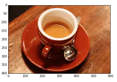
from skimage import ioimg=io.imread('d:/dog.jpg',as_grey=True)io.imshow(img) The program comes with pictures skimage The program comes with some sample pictures , If we don't want to read pictures from the outside , You can use these sample images directly :
astronaut Crew picture coffee A cup of coffee lena lena Beauty pictures camera Picture of the person with the camera coins Coin picture moon Moon picture checkerboard Chessboard picture horse Horse pictures page Page pictures chelsea Kitten picture hubble_deep_field Sky picture text Text image clock Clock picture immunohistochemistry Picture of colon The following code can be used to display these pictures , Without any parameters
from skimage import io, dataimg=data.lena()io.imshow(img)The image name corresponds to the function name , Such as camera The function name corresponding to the picture is camera(). These sample pictures are stored in skimage Under the installation directory of , The path name is data_dir, We can print out this path to see
from skimage import data_dirprint(data_dir) Save the picture Use io Modular imsave(fname,arr) Function to implement . The first parameter indicates the saved path and name , The second parameter represents the array variable to be saved .
from skimage import io,dataimg=data.chelsea()io.imshow(img)io.imsave('d:/cat.jpg',img)While saving the picture, it also plays a role in converting the format . If the image format when reading is jpg picture , Save as png Format , Then change the picture from jpg Convert the picture to png Picture and save .
Image pixel access and croppingAfter the picture is read into the program , In order to numpy Array exists . So right. numpy All the functions of array , It also applies to pictures . Access to array elements , In fact, it is the access to image pixels .
The access method of color pictures is :img[i,j,c]
i Indicates the number of lines in the picture ,j Represents the number of columns in the picture ,c Indicates the number of channels in the picture (RGB The three channels correspond to 0,1,2). The coordinates start from the upper left corner .
The gray image access method is :gray[i,j]
example 1: Output pictures of kittens G The... In the channel 20 That's ok 30 The pixel value of the column
from skimage import io,dataimg=data.chelsea()pixel=img[20,30,1]print(pixel)example 2: Show red single channel picture
from skimage import io,dataimg=data.chelsea()R=img[:,:,0]io.imshow(R)In addition to reading pixels , You can also modify pixel values .
example 3: Randomly add salt and pepper noise to kitten pictures
from skimage import io,dataimport numpy as npimg=data.chelsea()# Random generation 5000 Pepper and salt rows,cols,dims=img.shapefor i in range(5000): x=np.random.randint(0,rows) y=np.random.randint(0,cols) img[x,y,:]=255io.imshow(img)It's used here numpy In the bag random To generate random numbers ,randint(0,cols) Means to randomly generate an integer , The scope is 0 To cols Between .
use img[x,y,:]=255 This sentence is used to modify the pixel value , Change the original three channel pixel value , Turn into 255
By clipping the array , You can cut the picture .
example 4: Cut the kitten picture
from skimage import io,dataimg=data.chelsea()roi=img[80:180,100:200,:]io.imshow(roi)Operate on multiple pixels , Use array slicing to access . Slicing returns subscript access at a specified interval The pixel values of the array . Here are some examples of grayscale images :
img[i,:] = im[j,:] # Will be the first j The value of the row is assigned to i That's ok img[:,i] = 100 # Will be the first i All values of the column are set to 100img[:100,:50].sum() # Before calculation 100 That's ok 、 front 50 Column the sum of all the values img[50:100,50:100] # 50~100 That's ok ,50~100 Column ( Excluding the 100 Xing He 100 Column )img[i].mean() # The first i The average of all the values in the row img[:,-1] # The last column img[-2,:] (or im[-2]) # Second to last row Finally, let's look at two examples of accessing and changing pixel values :
example 5: take lena Binary image , The pixel value is greater than 128 Turn into 1, Otherwise it becomes 0
from skimage import io,data,colorimg=data.lena()img_gray=color.rgb2gray(img)rows,cols=img_gray.shapefor i in range(rows): for j in range(cols): if (img_gray[i,j]<=0.5): img_gray[i,j]=0 else: img_gray[i,j]=1io.imshow(img_gray)color Modular rgb2gray() function Used color Modular rgb2gray() function , Convert the color three channel picture into gray image . The result of the conversion is float64 An array of types , The scope is [0,1] Between .
Convert the color three channel picture into gray image , Finally become unit8, float Convert to unit8 There is a loss of information .
img_path = 'data/dpclassifier/newtrain/test/1_0.png'import Image as imgimport osfrom matplotlib import pyplot as plotfrom skimage import io,transform, img_as_ubyteimg_file1 = img.open(img_path)img_file1.show()img_file2 = io.imread(img_path)io.imshow(img_file2)print(type(img_file1),img_file1.mode, type(img_file2),img_file2.shape, img_file2.dtype,img_file2.max(),img_file2.min(),img_file2.mean())img_file22=skimage.color.rgb2gray(img_file2)print(type(img_file22),img_file22.shape,img_file22.dtype,img_file22.max(),img_file22.min(),img_file22.mean() )dst=img_as_ubyte(img_file22)print(type(dst),dst.shape,dst.dtype, dst.max(), dst.min(), dst.mean()) result (<class 'PIL.PngImagePlugin.PngImageFile'>, 'RGB', <type 'numpy.ndarray'>, (420, 512, 3), dtype('uint8'), 255, 0, 130.9983863467262)
(<type 'numpy.ndarray'>, (420, 512), dtype('float64'), 1.0, 0.0, 0.5137191621440242)
(<type 'numpy.ndarray'>, (420, 512), dtype('uint8'), 255, 0, 130.9983863467262)
example 6:
from skimage import io,dataimg=data.chelsea()reddish = img[:, :, 0] >170img[reddish] = [0, 255, 0]io.imshow(img)This example starts with R All pixel values of the channel , If it is greater than 170, Change the pixel value of this place to [0,255,0], namely G Channel value is 255,R and B Channel value is 0.
Image data type and color space conversionstay skimage in , A picture is a simple numpy Array , There are many data types for arrays , They can also be converted to each other . These data types and value ranges are shown in the following table :
Data type Rangeuint8 0 to 255uint16 0 to 65535uint32 0 to 232float -1 to 1 or 0 to 1int8 -128 to 127int16 -32768 to 32767int32 -231 to 231 - 1The pixel value range of a picture is [0,255], So the default type is unit8, The following code can be used to view the data type
from skimage import io,dataimg=data.chelsea()print(img.dtype.name)In the table above , Special note float type , Its scope is [-1,1] or [0,1] Between . After a color picture is converted into a gray image , Its type is determined by unit8 Turned into float
1、unit8 turn floatfrom skimage import data,img_as_floatimg=data.chelsea()print(img.dtype.name)dst=img_as_float(img)print(dst.dtype.name)2、float turn uint8from skimage import img_as_ubyteimport numpy as npimg = np.array([0, 0.5, 1], dtype=float)print(img.dtype.name)dst=img_as_ubyte(img)print(dst.dtype.name)float To unit8, It may cause data loss , So there will be warnings .*
In addition to the two most commonly used conversions , There are actually some other type conversions , The following table :
Function name Descriptionimg_as_float Convert to 64-bit floating point.img_as_ubyte Convert to 8-bit uint.img_as_uint Convert to 16-bit uint.img_as_int Convert to 16-bit int.As mentioned earlier , Except that direct conversion can change the data type , The data type can also be changed through the color space conversion of the image .
Common color spaces are Gray space 、rgb Space 、hsv Space and cmyk Space . After color space conversion , The types of pictures have become float type .
All color space conversion functions , All put in skimage Of color In module .
example :rgb Go to grayscale
from skimage import io,data,colorimg=data.lena()gray=color.rgb2gray(img)io.imshow(gray) Other conversions The usage is the same , List the common ones as follows :
skimage.color.rgb2grey(rgb)skimage.color.rgb2hsv(rgb)skimage.color.rgb2lab(rgb)skimage.color.gray2rgb(image)skimage.color.hsv2rgb(hsv)skimage.color.lab2rgb(lab)actually , All the above conversion functions , Can be replaced by a function
skimage.color.convert_colorspace(arr, fromspace, tospace)It means that you will arr from fromspace Color space to tospace Color space .
example :rgb turn hsv
from skimage import io,data,colorimg=data.lena()hsv=color.convert_colorspace(img,'RGB','HSV')io.imshow(hsv) stay color Module's color space conversion function , Another useful function is
skimage.color.label2rgb(arr), You can color the picture according to the tag value . In the future, this function can be used for coloring after image classification .
example : take lena Pictures fall into three categories , Then use the default color to shade the three categories
from skimage import io,data,colorimport numpy as npimg=data.lena()gray=color.rgb2gray(img)rows,cols=gray.shapelabels=np.zeros([rows,cols])for i in range(rows): for j in range(cols): if(gray[i,j]<0.4): labels[i,j]=0 elif(gray[i,j]<0.75): labels[i,j]=1 else: labels[i,j]=2dst=color.label2rgb(labels)io.imshow(dst) Drawing of image In fact, we have already used image rendering , Such as :
io.imshow(img) The essence of this line of code is to use matplotlib Package to draw pictures , After drawing successfully , Return to one matplotlib Data of type . therefore , We can also write :
import matplotlib.pyplot as pltplt.imshow(img)imshow() The function format is :
matplotlib.pyplot.imshow(X, cmap=None)X: The image or array to draw .
cmap: Color map (colormap), The default is to draw RGB(A) Color space .
Other optional color maps are listed below :
Color map describe
autumn red - orange - yellow
bone black - white ,x Line
cool green - Magenta
copper black - copper
flag red - white - blue - black
gray black - white
hot black - red - yellow - white
hsv hsv Color space , red - yellow - green - green - blue - Magenta - red
inferno black - red - yellow
jet blue - green - yellow - red
magma black - red - white
pink black - powder - white
plasma green - red - yellow
prism red - yellow - green - blue - purple -...- Green mode
spring Magenta - yellow
summer green - yellow
viridis blue - green - yellow
winter blue - green
There are a lot of gray,jet etc. , Such as :
plt.imshow(image,plt.cm.gray)plt.imshow(img,cmap=plt.cm.jet)After drawing the picture on the window , Return to one AxesImage object . To display this object in the window , We can call show() Function to display , But when practicing (ipython Environment ), Generally we can omit show() function , It can also be displayed automatically .
from skimage import io,dataimg=data.astronaut()dst=io.imshow(img)print(type(dst))io.show()You can see , The type is 'matplotlib.image.AxesImage'. Show a picture , We usually prefer to write :
import matplotlib.pyplot as pltfrom skimage import io,dataimg=data.astronaut()plt.imshow(img)plt.show()matplotlib It's a professional drawing library , amount to matlab Medium plot, You can set multiple figure window , Set up figure The title of the , Hide the ruler , You can even use subplot In a figure Show multiple pictures in . Generally, we can import matplotlib library :
import matplotlib.pyplot as pltin other words , We actually draw with matplotlib Bag pyplot modular .
use figure Functions and subplot Function to create three channels that separate the main window from the sub image and display the astronaut image at the same time
from skimage import dataimport matplotlib.pyplot as pltimg=data.astronaut()plt.figure(num='astronaut',figsize=(8,8)) # Create a file called astronaut The window of , And set the size plt.subplot(2,2,1) # Divide the window into two rows, two columns and four subgraphs , Four pictures can be displayed plt.title('origin image') # The title of the first picture plt.imshow(img) # Draw the first picture plt.subplot(2,2,2) # Second subgraph plt.title('R channel') # Title of the second picture plt.imshow(img[:,:,0],plt.cm.gray) # Draw the second picture , And it is a grayscale image plt.axis('off') # Do not show coordinate dimensions plt.subplot(2,2,3) # Third subgraph plt.title('G channel') # Title of the third picture plt.imshow(img[:,:,1],plt.cm.gray) # Draw the third picture , And it is a grayscale image plt.axis('off') # Do not show coordinate dimensions plt.subplot(2,2,4) # Fourth subgraph plt.title('B channel') # Title of the fourth picture plt.imshow(img[:,:,2],plt.cm.gray) # Draw the fourth picture , And it is a grayscale image plt.axis('off') # Do not show coordinate dimensions plt.show() # Display window In the process of drawing pictures , We use it matplotlib.pyplot Under the module of figure() Function to create a display window , The format of this function is :
matplotlib.pyplot.figure(num=None, figsize=None, dpi=None, facecolor=None, edgecolor=None)All parameters are optional , All have default values , Therefore, this function can be called without any parameters , among :
num: Integer or character type is OK . If set to integer , The integer number represents the sequence number of the window . If it is set to character type , The string represents the name of the window . Use this parameter to name the window , If two windows have the same serial number or name , Then the next window will overwrite the previous window .
figsize: Set window size . It's a tuple Integer of type , Such as figsize=(8,8)
dpi: Plastic figure , Represents the resolution of the window .
facecolor: The background color of the window .
edgecolor: Window border color .
use figure() Function to create a window , Only one picture can be displayed , If you want to display multiple pictures , You need to divide this window into several subgraphs , Show different pictures in each sub graph .
= We can use subplot() Function to partition subgraphs , The function format is :
matplotlib.pyplot.subplot(nrows, ncols, plot_number)nrows: Row number of subgraphs .
ncols: Number of columns in a subgraph .
plot_number: The number of the current subgraph .
Such as :
plt.subplot(2,2,1)Will be figure The window is divided into 2 That's ok 2 Columns were 4 Subtext , The present is the 1 Subtext . Sometimes we can use this kind of writing :
plt.subplot(221)The two writing methods have the same effect . The title of each subgraph is available title() Function to set , Whether to use coordinate ruler is available axis() Function to set , Such as :
plt.subplot(221)plt.title("first subwindow")plt.axis('off') use subplots To create display windows and partition subgraphs
In addition to the above method, create the display window and divide the subgraph , There is another way to write it , Here's an example :
import matplotlib.pyplot as pltfrom skimage import data,colorimg = data.immunohistochemistry()hsv = color.rgb2hsv(img)fig, axes = plt.subplots(2, 2, figsize=(7, 6))ax0, ax1, ax2, ax3 = axes.ravel()ax0.imshow(img)ax0.set_title("Original image")ax1.imshow(hsv[:, :, 0], cmap=plt.cm.gray)ax1.set_title("H")ax2.imshow(hsv[:, :, 1], cmap=plt.cm.gray)ax2.set_title("S")ax3.imshow(hsv[:, :, 2], cmap=plt.cm.gray)ax3.set_title("V")for ax in axes.ravel(): ax.axis('off')fig.tight_layout() # Automatic adjustment subplot Parameters between Direct use subplots() Function to create and divide windows . Be careful , It's better than the front subplot() One more function s, The format of this function is :
matplotlib.pyplot.subplots(nrows=1, ncols=1)
nrows: Number of rows of all subgraphs , The default is 1.
ncols: The number of all subgraphs , The default is 1.
Return to a window figure, And a tuple Type ax object , This object contains all the subgraphs , Can be combined with ravel() Function to list all subgraphs , Such as :
fig, axes = plt.subplots(2, 2, figsize=(7, 6))
ax0, ax1, ax2, ax3 = axes.ravel()
Created 2 That's ok 2 Column 4 Subtext , They are called ax0,ax1,ax2 and ax3, The title of each subgraph is set_title() Function to set , Such as :
ax0.imshow(img)
ax0.set_title("Original image")
If there are multiple subgraphs , We can also use tight_layout() Function to adjust the layout of the display , The format of this function is :
matplotlib.pyplot.tight_layout(pad=1.08, h_pad=None, w_pad=None, rect=None)All parameters are optional , All parameters can be omitted when calling this function .
pad: The distance between the edge of the main window and the edge of the subgraph , The default is 1.08
h_pad, w_pad: The distance between the edges of a subgraph , The default is pad_inches
rect: A rectangular area , If you set this value , Adjust all subgraphs to this rectangular area .
General call is :
plt.tight_layout() # Automatic adjustment subplot Parameters between Other methods of drawing and displaying Besides using matplotlib Library to draw pictures ,skimage There is another sub module viewer, A function is also provided to display the image . The difference is , It USES Qt Tool to create a canvas , To draw an image on the canvas .
example :
from skimage import datafrom skimage.viewer import ImageViewerimg = data.coins()viewer = ImageViewer(img)viewer.show()So to conclude , The functions commonly used to draw and display pictures are :
Function name function Invocation format figure Create a display window plt.figure(num=1,figsize=(8,8)imshow Drawing pictures plt.imshow(image)show Display window plt.show()subplot Divide the subgraphs plt.subplot(2,2,1)title Set the sub graph title ( And subplot Use a combination of ) plt.title('origin image')axis Whether to display the coordinate ruler plt.axis('off')subplots Create a window with multiple subgraphs fig,axes=plt.subplots(2,2,figsize=(8,8))ravel Set variables for each subgraph ax0,ax1,ax2,ax3=axes.ravel()set_title Set the sub graph title ( And axes Use a combination of ) ax0.set_title('first window')tight_layout Automatically adjust the sub graph display layout plt.tight_layout() Batch processing of images Sometimes , We don't just have to deal with a picture , Maybe a batch of pictures will be processed . Now , We can perform processing through loops , Can also call the program's own set of images to deal with .
The picture set function is :
skimage.io.ImageCollection(load_pattern,load_func=None) This function is placed in io In module , With two parameters , The first parameter load_pattern, Indicates the path of the picture group , It could be a str character string . The second parameter load_func Is a callback function , We can batch process images through this callback function . The callback function defaults to imread(), That is, the default function is to read pictures in batches .
Let's look at an example :
import skimage.io as iofrom skimage import data_dirstr=data_dir + '/*.png'coll = io.ImageCollection(str)print(len(coll))The result is 25, It means that the system comes with 25 Zhang png A sample picture of , These pictures have been read out , Put it in the picture collection coll in . If we want to show one of the pictures , You can add a line of code after it :
io.imshow(coll[10])Is shown as :
If a folder , We have some jpg Format picture , Some more png Format picture , Now I want to read them all , How do you do that ?
import skimage.io as iofrom skimage import data_dirstr='d:/pic/*.jpg:d:/pic/*.png'coll = io.ImageCollection(str)print(len(coll))Notice this place 'd:/pic/.jpg:d:/pic/.png' , Is a combination of two strings , The first is 'd:/pic/.jpg', The second is 'd:/pic/.png' , Together , The middle is separated by a colon , So we can take d:/pic/ Under folder jpg and png Format pictures are read out . If you want to read pictures stored in other places , It can also be added together , But the middle is also separated by colons .
io.ImageCollection() This function omits the second argument , That is, batch reading . If we don't want to read in bulk , But other batch operations , Such as batch conversion to grayscale image , So how to do it ?
You need to define a function first , Then take this function as the second argument , Such as :
from skimage import data_dir,io,colordef convert_gray(f): rgb=io.imread(f) return color.rgb2gray(rgb) str=data_dir+'/*.png'coll = io.ImageCollection(str,load_func=convert_gray)io.imshow(coll[10])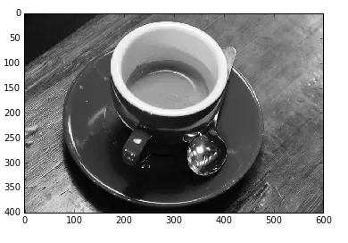
This batch operation is extremely useful for video processing , Because video is a series of pictures
from skimage import data_dir,io,colorclass AVILoader: video_file = 'myvideo.avi' def __call__(self, frame): return video_read(self.video_file, frame)avi_load = AVILoader()frames = range(0, 1000, 10) # 0, 10, 20, ...ic =io.ImageCollection(frames, load_func=avi_load) What this code means , Will be myvideo.avi Every... In this video 10 Frame picture read out , Put in the picture collection .
After getting the picture collection , We can also connect these pictures , Form a higher dimensional array , The function to connect pictures is :
skimage.io.concatenate_images(ic)With one parameter , Is the above picture collection , Such as :
from skimage import data_dir,io,colorcoll = io.ImageCollection('d:/pic/*.jpg')mat=io.concatenate_images(coll)Use concatenate_images(ic) The precondition of the function is that the size of the read pictures must be the same , Otherwise it will go wrong . Let's look at the dimensional changes before and after the picture connection :
from skimage import data_dir,io,colorcoll = io.ImageCollection('d:/pic/*.jpg')print(len(coll)) # Number of connected pictures print(coll[0].shape) # Picture size before connection , All the same mat=io.concatenate_images(coll)print(mat.shape) # Array size after connection Show results :
2
(870, 580, 3)
(2, 870, 580, 3)
You can see , take 2 individual 3 Dimension group , Connected into a 4 Dimension group
If we do batch operation on the pictures , You want to save the results after the operation , It can also be done .
example : Take all of the system's own png The sample picture , All converted to 256256 Of jpg Format grayscale , Save in d:/data/ Under the folder *
Change the size of the picture , We can use tranform Modular resize() function , This module will be discussed later .
from skimage import data_dir,io,transform,colorimport numpy as npdef convert_gray(f): rgb=io.imread(f) # Read... In turn rgb picture gray=color.rgb2gray(rgb) # take rgb Image to grayscale dst=transform.resize(gray,(256,256)) # Convert gray image size to 256*256 return dst str=data_dir+'/*.png'coll = io.ImageCollection(str,load_func=convert_gray)for i in range(len(coll)): io.imsave('d:/data/'+np.str(i)+'.jpg',coll[i]) # Cycle through saving pictures result :
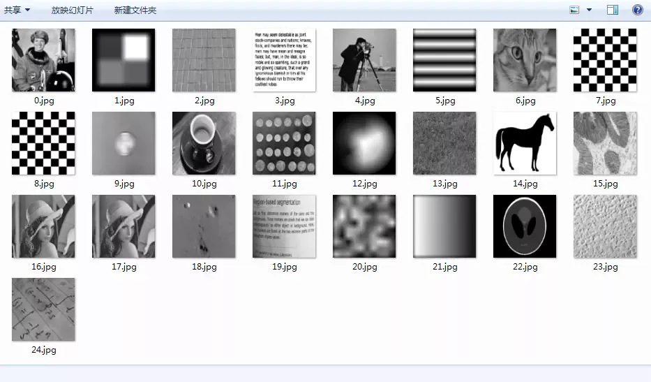
Image deformation and scaling , It uses skimage Of transform modular , There are many functions , The function is all ready .
1、 Change the picture size resizeThe function format is :
skimage.transform.resize(image, output_shape)image: Need to change the size of the picture
output_shape: New picture size
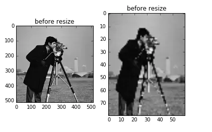
from skimage import transform,dataimport matplotlib.pyplot as pltimg = data.camera()dst=transform.resize(img, (80, 60))plt.figure('resize')plt.subplot(121)plt.title('before resize')plt.imshow(img,plt.cm.gray)plt.subplot(122)plt.title('before resize')plt.imshow(dst,plt.cm.gray)plt.show()take camera The picture is from the original 512x512 size , Turned into 80x60 size . From the coordinate ruler in the figure below , We can see :
The function format is :
skimage.transform.rescale(image, scale[, ...])scale Parameters can be single float Count , Represents the multiple of scaling , It can also be a float Type tuple, Such as [0.2,0.5], Means to scale the number of rows and columns separately
from skimage import transform,dataimg = data.camera()print(img.shape) # The original size of the picture print(transform.rescale(img, 0.1).shape) # Reduce to the size of the original picture 0.1print(transform.rescale(img, [0.5,0.25]).shape) # Reduce to half of the original picture lines , A quarter of the column print(transform.rescale(img, 2).shape) # Zoom in to the size of the original picture 2 times The result is :
3、 rotate rotate(512, 512)
(51, 51)
(256, 128)
(1024, 1024)
skimage.transform.rotate(image, angle[, ...],resize=False)angle The parameter is a float Number of types , Indicates the degree of rotation
resize Used to control when rotating , Whether to change the size , The default is False
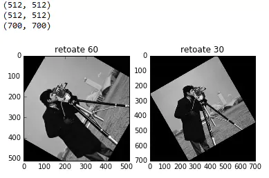
from skimage import transform,dataimport matplotlib.pyplot as pltimg = data.camera()print(img.shape) # The original size of the picture img1=transform.rotate(img, 60) # rotate 90 degree , Don't change the size print(img1.shape)img2=transform.rotate(img, 30,resize=True) # rotate 30 degree , Change the size at the same time print(img2.shape) plt.figure('resize')plt.subplot(121)plt.title('rotate 60')plt.imshow(img1,plt.cm.gray)plt.subplot(122)plt.title('rotate 30')plt.imshow(img2,plt.cm.gray)plt.show()Show results :
An effective but simple structure to interpret images with multi-resolution is the image pyramid . Image pyramid was originally used in machine vision and image compression , The pyramid of an image is a set of images arranged in a pyramid shape with gradually reduced resolution . At the bottom of the pyramid is a high-resolution representation of the image to be processed , And at the top is a low resolution approximation . When moving to the top of the pyramid , The size and resolution are reduced .
Here it is , Let's give an application example of Gaussian pyramid , The function prototype is :
skimage.transform.pyramid_gaussian(image, downscale=2)downscale Controls the scale of the pyramid
import numpy as npimport matplotlib.pyplot as pltfrom skimage import data,transformimage = data.astronaut() # Load astronaut pictures rows, cols, dim = image.shape # Get the number of lines of the picture , Number of columns and channels pyramid = tuple(transform.pyramid_gaussian(image, downscale=2)) # Generate Gaussian pyramid image # Symbiosis is log(512)=9 A pyramid image , Add original image total 10 picture ,pyramid[0]-pyramid[1]composite_image = np.ones((rows, cols + cols / 2, 3), dtype=np.double) # Generating background composite_image[:rows, :cols, :] = pyramid[0] # Fuse the original image i_row = 0for p in pyramid[1:]: n_rows, n_cols = p.shape[:2] composite_image[i_row:i_row + n_rows, cols:cols + n_cols] = p # Cycle fusion 9 A pyramid image i_row += n_rowsplt.imshow(composite_image)plt.show()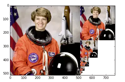
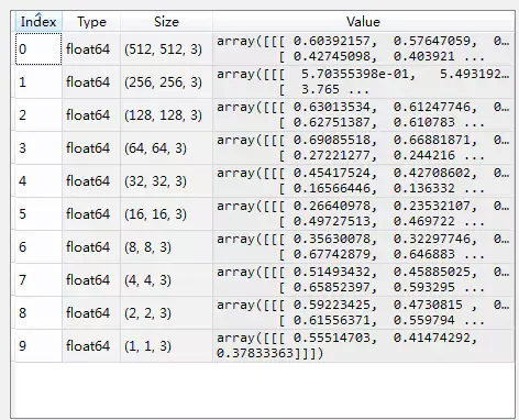
Top right , Namely 10 A pyramid image , Subscript to be 0 Represents the original image , The image rows and columns of each subsequent layer become half of the previous layer , Until it becomes 1
Except for the Gauss pyramid , There are other pyramids , Such as :
skimage.transform.pyramid_laplacian(image, downscale=2)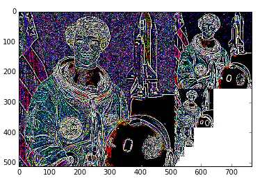
Adjustment of image brightness and contrast , It's on the skimage Bag exposure Inside the module
1、gamma adjustmentprinciple :I=Ig
For the pixels of the original image , Perform power operation , Get the new pixel value . Formula g Namely gamma value .
If gamma>1, The new image is darker than the original image
If gamma<1, The new image is brighter than the original image
The function format is :
skimage.exposure.adjust_gamma(image, gamma=1)gamma The parameter defaults to 1, The original image does not change .
from skimage import data, exposure, img_as_floatimport matplotlib.pyplot as pltimage = img_as_float(data.moon())gam1= exposure.adjust_gamma(image, 2) # Dimming gam2= exposure.adjust_gamma(image, 0.5) # Dimming plt.figure('adjust_gamma',figsize=(8,8))plt.subplot(131)plt.title('origin image')plt.imshow(image,plt.cm.gray)plt.axis('off')plt.subplot(132)plt.title('gamma=2')plt.imshow(gam1,plt.cm.gray)plt.axis('off')plt.subplot(133)plt.title('gamma=0.5')plt.imshow(gam2,plt.cm.gray)plt.axis('off')plt.show()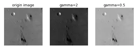
This is just like gamma contrary
principle :I=log(I)
from skimage import data, exposure, img_as_floatimport matplotlib.pyplot as pltimage = img_as_float(data.moon())gam1= exposure.adjust_log(image) # Logarithmic adjustment plt.figure('adjust_gamma',figsize=(8,8))plt.subplot(121)plt.title('origin image')plt.imshow(image,plt.cm.gray)plt.axis('off')plt.subplot(122)plt.title('log')plt.imshow(gam1,plt.cm.gray)plt.axis('off')plt.show()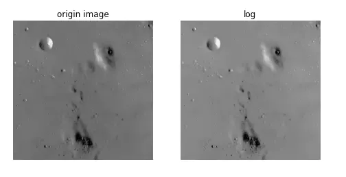
function :is_low_contrast(img)
Return to one bool Type value
from skimage import data, exposureimage =data.moon()result=exposure.is_low_contrast(image)print(result)Output is False
4、 Adjust the intensityfunction :
skimage.exposure.rescale_intensity(image, in_range='image', out_range='dtype')in_range Indicates the intensity range of the input picture , The default is 'image', Represents the maximum size of the image / The minimum pixel value is used as the range
out_range Indicates the intensity range of the output picture , The default is 'dype', Represents the maximum of the type of image used / The minimum value is used as the range
By default , Enter the name of the picture [min,max] The range is stretched to [dtype.min, dtype.max], If dtype=uint8, that dtype.min=0, dtype.max=255
import numpy as npfrom skimage import exposureimage = np.array([51, 102, 153], dtype=np.uint8)mat=exposure.rescale_intensity(image)print(mat)Output is [ 0 127 255]
That is, the minimum pixel value is determined by 51 Turn into 0, The maximum value is determined by 153 Turn into 255, The whole is stretched , But the data type has not changed , still uint8
We talked about , Can pass img_as_float() Function will unit8 Type conversion to float type , There are actually simpler ways , It's times 1.0
import numpy as npimage = np.array([51, 102, 153], dtype=np.uint8)print(image*1.0)by [51,102,153] Turned into [ 51. 102. 153.]
and float The range of types is [0,1], So right. float Conduct rescale_intensity After the adjustment , Range becomes [0,1], instead of [0,255]
import numpy as npfrom skimage import exposureimage = np.array([51, 102, 153], dtype=np.uint8)tmp=image*1.0mat=exposure.rescale_intensity(tmp)print(mat)The result is [ 0. 0.5 1. ]
If the original pixel value does not want to be stretched , Just wait for the scale to shrink , Just use in_range Parameters , Such as :
import numpy as npfrom skimage import exposureimage = np.array([51, 102, 153], dtype=np.uint8)tmp=image*1.0mat=exposure.rescale_intensity(tmp,in_range=(0,255))print(mat)Output is :[ 0.2 0.4 0.6], That is, the original pixel value is divided by 255
If parameters in_range Of [main,max] The range is larger than the range of the original pixel value [min,max] Big or small , Then cut it , Such as :
mat=exposure.rescale_intensity(tmp,in_range=(0,102))print(mat)Output [ 0.5 1. 1. ], That is, the original pixel value is divided by 102, beyond 1 Turn into 1
If there are negative numbers in an array , Now I want to adjust to a positive number , Just use out_range Parameters . Such as :
import numpy as npfrom skimage import exposureimage = np.array([-10, 0, 10], dtype=np.int8)mat=exposure.rescale_intensity(image, out_range=(0, 127))print(mat)Histogram and equalizationOutput [ 0 63 127]
In image processing , Histogram is very important , It is also a very useful processing element .
stay skimage Histogram processing in the library , It's on the exposure In this module .
1、 Calculate the histogram function :
skimage.exposure.histogram(image, nbins=256)stay numpy In bag , It also provides a function to calculate the histogram histogram(), The two have the same meaning .
Return to one tuple(hist, bins_center), The previous array is the statistics of the histogram , The latter array is each bin The middle value of
import numpy as npfrom skimage import exposure,dataimage =data.camera()*1.0hist1=np.histogram(image, bins=2) # use numpy Packet calculation histogram hist2=exposure.histogram(image, nbins=2) # use skimage Calculate the histogram print(hist1)print(hist2)Output :
(array([107432, 154712], dtype=int64), array([ 0. , 127.5, 255. ]))
(array([107432, 154712], dtype=int64), array([ 63.75, 191.25]))
Divided into two groups. bin, Every bin The statistics are the same , but numpy It's every bin Range values at both ends of , and skimage It's every bin The middle value of
2、 Draw histogramDrawing can call matplotlib.pyplot Library for , Among them hist Function can draw histogram directly .
Call mode :
n, bins, patches = plt.hist(arr, bins=10, normed=0, facecolor='black', edgecolor='black',alpha=1,histtype='bar')hist Many parameters , But these are the six commonly used , Only the first one is necessary , The last four options
arr: Need to calculate a one-dimensional array of histograms bins: Number of columns of histogram , optional , The default is 10normed: Whether to normalize the obtained histogram vector . The default is 0facecolor: Histogram color edgecolor: Histogram border color alpha: transparency histtype: Histogram Type ,‘bar', ‘barstacked', ‘step', ‘stepfilled'Return value :
n: Histogram vector , Whether to normalize by parameter normed Set up bins: Return to each bin Range of patches: Return each bin Data contained in it , It's a listfrom skimage import dataimport matplotlib.pyplot as pltimg=data.camera()plt.figure("hist")arr=img.flatten()n, bins, patches = plt.hist(arr, bins=256, normed=1,edgecolor='None',facecolor='red') plt.show()
Among them flatten() The function is numpy The inside of the bag , Used to serialize a two-dimensional array into a one-dimensional array .
Is a sequence of lines , Such as
mat=[[1 2 3 4 5 6]]after mat.flatten() after , It becomes
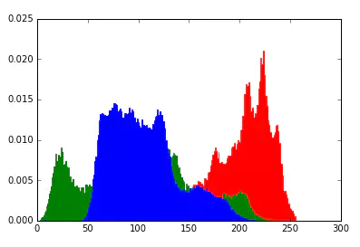
mat=[1 2 3 4 5 6]3、 Color picture three channel histogram Generally speaking, histograms are characteristic pairs of grayscale images , If you want to draw rgb Three channel histogram of image , In fact, it is the superposition of three histograms .
from skimage import dataimport matplotlib.pyplot as pltimg=data.lena()ar=img[:,:,0].flatten()plt.hist(ar, bins=256, normed=1,facecolor='r',edgecolor='r',hold=1)ag=img[:,:,1].flatten()plt.hist(ag, bins=256, normed=1, facecolor='g',edgecolor='g',hold=1)ab=img[:,:,2].flatten()plt.hist(ab, bins=256, normed=1, facecolor='b',edgecolor='b')plt.show()among , Add a parameter hold=1, Indicates that it can be superimposed
If the pixels of an image occupy many gray levels and are evenly distributed , Then such images often have high contrast and changeable gray tones . Histogram equalization is a transformation function that can automatically achieve this effect only by inputting image histogram information . Its basic idea is to widen the gray level with more pixels in the image , The gray scale with a small number of pixels in the image is compressed , So as to expand the dynamic range of values , Improved contrast and gray tone changes , Make the image clearer .
from skimage import data,exposureimport matplotlib.pyplot as pltimg=data.moon()plt.figure("hist",figsize=(8,8))arr=img.flatten()plt.subplot(221)plt.imshow(img,plt.cm.gray) # original image plt.subplot(222)plt.hist(arr, bins=256, normed=1,edgecolor='None',facecolor='red') # Histogram of original image img1=exposure.equalize_hist(img)arr1=img1.flatten()plt.subplot(223)plt.imshow(img1,plt.cm.gray) # Equalize image plt.subplot(224)plt.hist(arr1, bins=256, normed=1,edgecolor='None',facecolor='red') # Equalization histogram plt.show()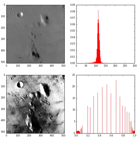
skimage.exposure.``equalize_adapthist(image, kernel_size=None, clip_limit=0.01, nbins=256)
Contrast Limited Adaptive Histogram Equalization (CLAHE).
An algorithm for local contrast enhancement, that uses histograms computed over different tile regions of the image. Local details can therefore be enhanced even in regions that are darker or lighter than most of the image.
image : (M, N[, C]) ndarray
Input image.
kernel_size: integer or list-like, optionalDefines the shape of contextual regions used in the algorithm. If iterable is passed, it must have the same number of elements asimage.ndim(without color channel). If integer, it is broadcasted to each image dimension. By default,kernel_sizeis 1/8 ofimageheight by 1/8 of its width.
clip_limit : float, optional
Clipping limit, normalized between 0 and 1 (higher values give more contrast).
nbins : int, optional
Number of gray bins for histogram (“data range”).
| Returns: |
out : (M, N[, C]) ndarray
Equalized image.
http://scikit-image.org/docs/dev/api/skimage.exposure.html#equalize-adapthist
from skimage import data,exposureimport matplotlib.pyplot as plt#%matplotlib notebookclip_limitnumber=0.01img=data.moon()print(img.shape)plt.figure("hist",figsize=(8,8))arr=img.flatten()plt.subplot(5,2,1)plt.title('original')plt.imshow(img,plt.cm.gray) # original image plt.subplot(5,2,2)plt.hist(arr, bins=256, normed=1,edgecolor='None',facecolor='red') # Histogram of original image # #img1=exposure.equalize_hist(img)# img1=exposure.equalize_hist(img)# arr1=img1.flatten()# plt.subplot(6,2,3)# plt.title('equalize_hist')# plt.imshow(img1,plt.cm.gray) # Equalize image # plt.subplot(6,2,4)# plt.hist(arr1, bins=256, normed=1,edgecolor='None',facecolor='red') # Equalization histogram # plt.show()img2=exposure.equalize_adapthist(img, kernel_size=256, clip_limit=clip_limitnumber, nbins=256)arr2=img2.flatten()plt.subplot(5,2,3)plt.title('equalize_adapthist-256-'+ str(clip_limitnumber))plt.imshow(img2,plt.cm.gray) # Equalize image plt.subplot(5,2,4)plt.hist(arr2, bins=256, normed=1,edgecolor='None',facecolor='red') # Equalization histogram plt.show()img3=exposure.equalize_adapthist(img, kernel_size=128, clip_limit=clip_limitnumber, nbins=256)arr3=img3.flatten()plt.subplot(5,2,5)plt.title('equalize_adapthist-128-'+ str(clip_limitnumber))plt.imshow(img3,plt.cm.gray) # Equalize image plt.subplot(5,2,6)plt.hist(arr3, bins=256, normed=1,edgecolor='None',facecolor='red') # Equalization histogram plt.show()img4=exposure.equalize_adapthist(img, kernel_size=64, clip_limit=clip_limitnumber, nbins=256)arr4=img4.flatten()plt.subplot(5,2,7)plt.title('equalize_adapthist-64-'+ str(clip_limitnumber))plt.imshow(img4,plt.cm.gray) # Equalize image plt.subplot(5,2,8)plt.hist(arr4, bins=256, normed=1,edgecolor='None',facecolor='red') # Equalization histogram plt.show()img5=exposure.equalize_adapthist(img, kernel_size=32, clip_limit=clip_limitnumber, nbins=256)arr5=img5.flatten()plt.subplot(5,2,9)plt.title('equalize_adapthist-32-'+ str(clip_limitnumber))plt.imshow(img5,plt.cm.gray) # Equalize image plt.subplot(5,2,10)plt.hist(arr5, bins=256, normed=1,edgecolor='None',facecolor='red') # Equalization histogram plt.show()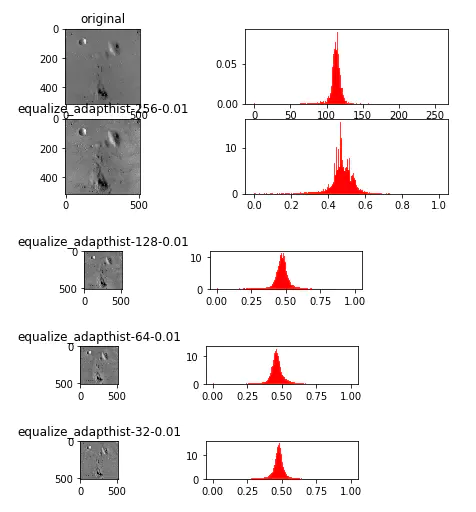
1.png
from skimage import data,exposureimport matplotlib.pyplot as plt#%matplotlib notebookkernel_sizenuber=64img=data.moon()print(img.shape)plt.figure("hist",figsize=(8,8))arr=img.flatten()plt.subplot(5,2,1)plt.title('original')plt.imshow(img,plt.cm.gray) # original image plt.subplot(5,2,2)plt.hist(arr, bins=256, normed=1,edgecolor='None',facecolor='red') # Histogram of original image # #img1=exposure.equalize_hist(img)# img1=exposure.equalize_hist(img)# arr1=img1.flatten()# plt.subplot(6,2,3)# plt.title('equalize_hist')# plt.imshow(img1,plt.cm.gray) # Equalize image # plt.subplot(6,2,4)# plt.hist(arr1, bins=256, normed=1,edgecolor='None',facecolor='red') # Equalization histogram # plt.show()img2=exposure.equalize_adapthist(img, kernel_size=kernel_sizenuber, clip_limit=0.001, nbins=256)arr2=img2.flatten()plt.subplot(5,2,3)plt.title('equalize_adapthist-'+ str(kernel_sizenuber)+'-0.001')plt.imshow(img2,plt.cm.gray) # Equalize image plt.subplot(5,2,4)plt.hist(arr2, bins=256, normed=1,edgecolor='None',facecolor='red') # Equalization histogram plt.show()img3=exposure.equalize_adapthist(img, kernel_size=kernel_sizenuber, clip_limit=0.005, nbins=256)arr3=img3.flatten()plt.subplot(5,2,5)plt.title('equalize_adapthist-'+ str(kernel_sizenuber)+'-0.005')plt.imshow(img3,plt.cm.gray) # Equalize image plt.subplot(5,2,6)plt.hist(arr3, bins=256, normed=1,edgecolor='None',facecolor='red') # Equalization histogram plt.show()img4=exposure.equalize_adapthist(img, kernel_size=kernel_sizenuber, clip_limit=0.01, nbins=256)arr4=img4.flatten()plt.subplot(5,2,7)plt.title('equalize_adapthist-'+ str(kernel_sizenuber)+'-0.01')plt.imshow(img4,plt.cm.gray) # Equalize image plt.subplot(5,2,8)plt.hist(arr4, bins=256, normed=1,edgecolor='None',facecolor='red') # Equalization histogram plt.show()img5=exposure.equalize_adapthist(img, kernel_size=kernel_sizenuber, clip_limit=0.05, nbins=256)arr5=img5.flatten()plt.subplot(5,2,9)plt.title('equalize_adapthist-'+ str(kernel_sizenuber)+'-0.05')plt.imshow(img5,plt.cm.gray) # Equalize image plt.subplot(5,2,10)plt.hist(arr5, bins=256, normed=1,edgecolor='None',facecolor='red') # Equalization histogram plt.show()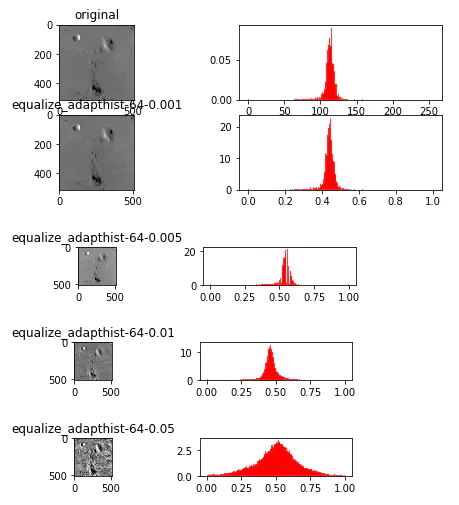
reference
python digital image processing
That's all python skimage Details of image processing , More about python skimage For information on image processing, please pay attention to other relevant articles on the software development network !