Data transferred from (GitHub Address ):https://github.com/wesm/pydata-book Friends in need can go by themselves github download 
This chapter includes a few messy chapters , You don't need to study it carefully .
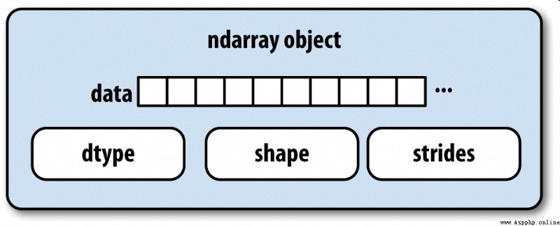
NumPy Of ndarray It provides a way to integrate homogeneous data blocks ( It can be continuous or across ) How to interpret as a multidimensional array object . As you have seen before , data type (dtype) Determines how the data is interpreted , Floating point numbers, for example 、 Integers 、 Boolean value, etc .
ndarray Part of the reason why this is so powerful is that all array objects are a spanning view of data blocks (strided view). You might want to know about array views arr[::2,::-1] Why not replicate any data . In short ,ndarray Not just a piece of memory and a dtype, It also has span information , This allows the array to move in various steps (step size) Move in memory . To be more precise ,ndarray The interior consists of :
chart A-1 It simply explains ndarray The internal structure of .
for example , One 10×5 Array of , Its shape is (10,5):
In [10]: np.ones((10, 5)).shape
Out[10]: (10, 5)
A typical (C The order , We will explain in detail later )3×4×5 Of float64(8 Bytes ) Array , Its span is (160,40,8) —— Knowing the span is very useful , Usually , The larger the span on one axis , The more expensive it is to compute along this axis :
In [11]: np.ones((3, 4, 5), dtype=np.float64).strides
Out[11]: (160, 40, 8)
although NumPy Users are rarely interested in array span information , But they are important factors in building non - replicated array views . The span can even be negative , This causes the array to move backward in memory , Like slicing obj[::-1] or obj[:,::-1] That's what happened in China .
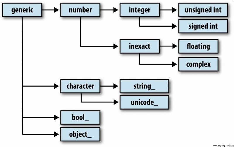
You may occasionally need to check whether an array contains integers 、 Floating point numbers 、 String or Python object . Because there are many kinds of floating point numbers ( from float16 To float128), Judge dtype Whether it belongs to a certain category is very tedious . Fortunately, ,dtype Have a superclass ( such as np.integer and np.floating), They can follow np.issubdtype Function in combination with :
In [12]: ints = np.ones(10, dtype=np.uint16)
In [13]: floats = np.ones(10, dtype=np.float32)
In [14]: np.issubdtype(ints.dtype, np.integer)
Out[14]: True
In [15]: np.issubdtype(floats.dtype, np.floating)
Out[15]: True
call dtype Of mro Method to view all its parent classes :
In [16]: np.float64.mro()
Out[16]:
[numpy.float64,
numpy.floating,
numpy.inexact,
numpy.number,
numpy.generic,
float,
object]
Then get :
In [17]: np.issubdtype(ints.dtype, np.number)
Out[17]: True
Most of the NumPy Users do not need to know this knowledge at all , But this knowledge can come in handy occasionally . chart A-2 Illustrates the dtype System and parent-child relationship .
Divide the fancy index 、 section 、 Boolean condition subset and other operations , There are many other ways to manipulate arrays . although pandas The advanced functions in can handle many heavy tasks in data analysis , But sometimes you still need to write some data algorithms that can't be found in the existing library .
Most of the time , You don't have to copy any data , Just convert the array from one shape to another . Just add an instance method to the array reshape This can be achieved by passing in a tuple representing the new shape . for example , Suppose you have a one-dimensional array , We want to rearrange it into a matrix ( The results are shown in the figure A-3):
In [18]: arr = np.arange(8)
In [19]: arr
Out[19]: array([0, 1, 2, 3, 4, 5, 6, 7])
In [20]: arr.reshape((4, 2))
Out[20]:
array([[0, 1],
[2, 3],
[4, 5],
[6, 7]])
Multidimensional arrays can also be reshaped :
In [21]: arr.reshape((4, 2)).reshape((2, 4))
Out[21]:
array([[0, 1, 2, 3],
[4, 5, 6, 7]])
One dimension of the shape as a parameter can be -1, It indicates that the size of the dimension is inferred from the data itself :
In [22]: arr = np.arange(15)
In [23]: arr.reshape((5, -1))
Out[23]:
array([[ 0, 1, 2],
[ 3, 4, 5],
[ 6, 7, 8],
[ 9, 10, 11],
[12, 13, 14]])
And reshape Converting a one-dimensional array into a multi-dimensional array is usually called flattening (flattening) Or spread out (raveling):
In [27]: arr = np.arange(15).reshape((5, 3))
In [28]: arr
Out[28]:
array([[ 0, 1, 2],
[ 3, 4, 5],
[ 6, 7, 8],
[ 9, 10, 11],
[12, 13, 14]])
In [29]: arr.ravel()
Out[29]: array([ 0, 1, 2, 3, 4, 5, 6, 7, 8, 9, 10, 11, 12, 13, 14])
If the value in the result is the same as the original array ,ravel No copy of the source data will be generated .flatten Methods behave like ravel, But it always returns a copy of the data :
In [30]: arr.flatten()
Out[30]: array([ 0, 1, 2, 3, 4, 5, 6, 7, 8, 9, 10, 11, 12, 13, 14])
Arrays can be reshaped or spread out in other order . This is right NumPy It's a delicate problem for beginners , So in the next section, we will focus on this problem .
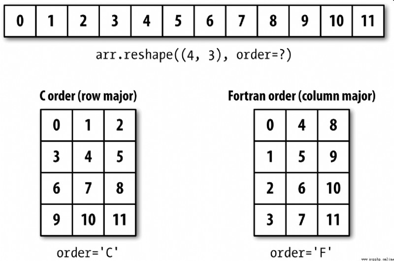
NumPy It allows you to control the layout of data in memory more flexibly . By default ,NumPy Arrays are created in row first order . In terms of space , That means , For a two-dimensional array , The data items in each row are stored in adjacent memory locations . Another order is column priority , It means that the data items in each column are stored in adjacent memory locations .
For some historical reasons , Row and column priorities are also called... Respectively C and Fortran The order . stay FORTRAN 77 in , Matrices are all column first .
image reshape and reval A function like this , Can accept a that represents the storage order of array data order Parameters . It can generally be ’C’ or ’F’( also ’A’ and ’K’ And so on , Please refer to NumPy Documents ). chart A-3 This is explained :
In [31]: arr = np.arange(12).reshape((3, 4))
In [32]: arr
Out[32]:
array([[ 0, 1, 2, 3],
[ 4, 5, 6, 7],
[ 8, 9, 10, 11]])
In [33]: arr.ravel()
Out[33]: array([ 0, 1, 2, 3, 4, 5, 6, 7, 8, 9, 10, 11])
In [34]: arr.ravel('F')
Out[34]: array([ 0, 4, 8, 1, 5, 9, 2, 6, 10, 3, 7, 11])
The process of reshaping a two-dimensional or higher dimensional array is rather puzzling ( See the picture A-3).C and Fortran The key difference in order is the order in which dimensions travel :
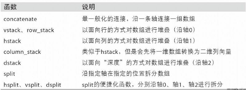
numpy.concatenate A sequence consisting of an array can be divided by a specified axis ( As tuple 、 List etc. ) Connect together :
In [35]: arr1 = np.array([[1, 2, 3], [4, 5, 6]])
In [36]: arr2 = np.array([[7, 8, 9], [10, 11, 12]])
In [37]: np.concatenate([arr1, arr2], axis=0)
Out[37]:
array([[ 1, 2, 3],
[ 4, 5, 6],
[ 7, 8, 9],
[10, 11, 12]])
In [38]: np.concatenate([arr1, arr2], axis=1)
Out[38]:
array([[ 1, 2, 3, 7, 8, 9],
[ 4, 5, 6, 10, 11, 12]])
For common connection operations ,NumPy Some convenient methods are provided ( Such as vstack and hstack). therefore , The above operation can also be expressed as :
In [39]: np.vstack((arr1, arr2))
Out[39]:
array([[ 1, 2, 3],
[ 4, 5, 6],
[ 7, 8, 9],
[10, 11, 12]])
In [40]: np.hstack((arr1, arr2))
Out[40]:
array([[ 1, 2, 3, 7, 8, 9],
[ 4, 5, 6, 10, 11, 12]])
On the contrary ,split Used to split an array into multiple arrays along a specified axis :
In [41]: arr = np.random.randn(5, 2)
In [42]: arr
Out[42]:
array([[-0.2047, 0.4789],
[-0.5194, -0.5557],
[ 1.9658, 1.3934],
[ 0.0929, 0.2817],
[ 0.769 , 1.2464]])
In [43]: first, second, third = np.split(arr, [1, 3])
In [44]: first
Out[44]: array([[-0.2047, 0.4789]])
In [45]: second
Out[45]:
array([[-0.5194, -0.5557],
[ 1.9658, 1.3934]])
In [46]: third
Out[46]:
array([[ 0.0929, 0.2817],
[ 0.769 , 1.2464]])
The incoming to np.split Value [1,3] Indicates at which index the array is split .
surface A-1 All functions for array join and split are listed in , Some of them are specially provided to facilitate common connection operations .
NumPy There are two special objects in the namespace ——r_ and c_, They can make the stacking operation of arrays more concise :
In [47]: arr = np.arange(6)
In [48]: arr1 = arr.reshape((3, 2))
In [49]: arr2 = np.random.randn(3, 2)
In [50]: np.r_[arr1, arr2]
Out[50]:
array([[ 0. , 1. ],
[ 2. , 3. ],
[ 4. , 5. ],
[ 1.0072, -1.2962],
[ 0.275 , 0.2289],
[ 1.3529, 0.8864]])
In [51]: np.c_[np.r_[arr1, arr2], arr]
Out[51]:
array([[ 0. , 1. , 0. ],
[ 2. , 3. , 1. ],
[ 4. , 5. , 2. ],
[ 1.0072, -1.2962, 3. ],
[ 0.275 , 0.2289, 4. ],
[ 1.3529, 0.8864, 5. ]])
It can also convert slices into arrays :
In [52]: np.c_[1:6, -10:-5]
Out[52]:
array([[ 1, -10],
[ 2, -9],
[ 3, -8],
[ 4, -7],
[ 5, -6]])
r_ and c_ Please refer to its documentation for specific functions .
The main tools for repeating arrays to produce larger arrays are repeat and tile These two functions .repeat Each element in the array will be repeated a certain number of times , This produces a larger array :
In [53]: arr = np.arange(3)
In [54]: arr
Out[54]: array([0, 1, 2])
In [55]: arr.repeat(3)
Out[55]: array([0, 0, 0, 1, 1, 1, 2, 2, 2])
note : With other popular array programming languages ( Such as MATLAB) Different ,NumPy You rarely need to repeat an array in (replicate). This is mainly because of the broadcast (broadcasting, We will explain this technique in the next section ) Can better meet this demand .
By default , If you pass in an integer , Then each element will repeat that many times . If you pass in a set of integers , Then each element can be repeated for different times :
In [56]: arr.repeat([2, 3, 4])
Out[56]: array([0, 0, 1, 1, 1, 2, 2, 2, 2])
For multidimensional arrays , You can also make their elements repeat along a specified axis :
In [57]: arr = np.random.randn(2, 2)
In [58]: arr
Out[58]:
array([[-2.0016, -0.3718],
[ 1.669 , -0.4386]])
In [59]: arr.repeat(2, axis=0)
Out[59]:
array([[-2.0016, -0.3718],
[-2.0016, -0.3718],
[ 1.669 , -0.4386],
[ 1.669 , -0.4386]])
Be careful , If the axial direction is not set , The array will be flattened , This may not be the result you want . Again , When repeating a multi dimension , You can also pass in a set of integers , This will cause each slice to repeat a different number of times :
In [60]: arr.repeat([2, 3], axis=0)
Out[60]:
array([[-2.0016, -0.3718],
[-2.0016, -0.3718],
[ 1.669 , -0.4386],
[ 1.669 , -0.4386],
[ 1.669 , -0.4386]])
In [61]: arr.repeat([2, 3], axis=1)
Out[61]:
array([[-2.0016, -2.0016, -0.3718, -0.3718, -0.3718],
[ 1.669 , 1.669 , -0.4386, -0.4386, -0.4386]])
tile The function of is to stack copies of an array along a specified axis . You can visualize it as “ Tiling ”:
In [62]: arr
Out[62]:
array([[-2.0016, -0.3718],
[ 1.669 , -0.4386]])
In [63]: np.tile(arr, 2)
Out[63]:
array([[-2.0016, -0.3718, -2.0016, -0.3718],
[ 1.669 , -0.4386, 1.669 , -0.4386]])
The second parameter is the number of tiles . For scalars , The tiles are laid horizontally , Instead of laying vertically . It can be a representation of “ layout ” Tuple of layout :
In [64]: arr
Out[64]:
array([[-2.0016, -0.3718],
[ 1.669 , -0.4386]])
In [65]: np.tile(arr, (2, 1))
Out[65]:
array([[-2.0016, -0.3718],
[ 1.669 , -0.4386],
[-2.0016, -0.3718],
[ 1.669 , -0.4386]])
In [66]: np.tile(arr, (3, 2))
Out[66]:
array([[-2.0016, -0.3718, -2.0016, -0.3718],
[ 1.669 , -0.4386, 1.669 , -0.4386],
[-2.0016, -0.3718, -2.0016, -0.3718],
[ 1.669 , -0.4386, 1.669 , -0.4386],
[-2.0016, -0.3718, -2.0016, -0.3718],
[ 1.669 , -0.4386, 1.669 , -0.4386]])
In the 4 In chapter, we talked about , One way to get and set a subset of an array is to use fancy indexes through integer arrays :
In [67]: arr = np.arange(10) * 100
In [68]: inds = [7, 1, 2, 6]
In [69]: arr[inds]
Out[69]: array([700, 100, 200, 600])
ndarray There are other methods for obtaining a single axial selection :
In [70]: arr.take(inds)
Out[70]: array([700, 100, 200, 600])
In [71]: arr.put(inds, 42)
In [72]: arr
Out[72]: array([ 0, 42, 42, 300, 400, 500, 42, 42,800, 900])
In [73]: arr.put(inds, [40, 41, 42, 43])
In [74]: arr
Out[74]: array([ 0, 41, 42, 300, 400, 500, 43, 40, 800, 900])
To be used on other shafts take, Just incoming axis Key words can be used :
In [75]: inds = [2, 0, 2, 1]
In [76]: arr = np.random.randn(2, 4)
In [77]: arr
Out[77]:
array([[-0.5397, 0.477 , 3.2489, -1.0212],
[-0.5771, 0.1241, 0.3026, 0.5238]])
In [78]: arr.take(inds, axis=1)
Out[78]:
array([[ 3.2489, -0.5397, 3.2489, 0.477 ],
[ 0.3026, -0.5771, 0.3026, 0.1241]])
put Don't accept axis Parameters , It will only be in the flattened version of the array ( A one-dimensional ,C The order ) Index on . therefore , When you need to set elements with other axial indexes , Better to use fancy indexes .
radio broadcast (broadcasting) It refers to the execution of arithmetic operations between arrays of different shapes . It is a very powerful function , But it's also misleading , Even experienced veterans . The simplest broadcast occurs when you combine scalar values with arrays :
In [79]: arr = np.arange(5)
In [80]: arr
Out[80]: array([0, 1, 2, 3, 4])
In [81]: arr * 4
Out[81]: array([ 0, 4, 8, 12, 16])
Here we say : In this multiplication , Scalar values 4 Broadcast to all other elements .
Take an example , We can flatten each column of the array by subtracting the column average . It's a very simple problem to solve :
In [82]: arr = np.random.randn(4, 3)
In [83]: arr.mean(0)
Out[83]: array([-0.3928, -0.3824, -0.8768])
In [84]: demeaned = arr - arr.mean(0)
In [85]: demeaned
Out[85]:
array([[ 0.3937, 1.7263, 0.1633],
[-0.4384, -1.9878, -0.9839],
[-0.468 , 0.9426, -0.3891],
[ 0.5126, -0.6811, 1.2097]])
In [86]: demeaned.mean(0)
Out[86]: array([-0., 0., -0.])
chart A-4 This process is vividly demonstrated . It will be a little troublesome to flatten rows by broadcasting . Fortunately, , Just follow certain rules , Low dimensional values can be broadcast to any dimension of the array ( For example, subtract the row average value from each column of a two-dimensional array ).
So I got :

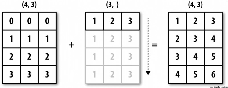
Although I am an experienced NumPy an old hand , But often you have to stop and draw a picture and think about the principles of broadcasting . Let's look at the last example , Suppose you want to subtract that average from each row . because arr.mean(0) The length of is 3, So it can be in 0 Broadcast axially : because arr The trailing edge dimension of is 3, So they are compatible . According to the principle , To be in 1 Subtract axially ( That is, subtract the line average from each line ), The shape of the smaller array must be (4,1):
In [87]: arr
Out[87]:
array([[ 0.0009, 1.3438, -0.7135],
[-0.8312, -2.3702, -1.8608],
[-0.8608, 0.5601, -1.2659],
[ 0.1198, -1.0635, 0.3329]])
In [88]: row_means = arr.mean(1)
In [89]: row_means.shape
Out[89]: (4,)
In [90]: row_means.reshape((4, 1))
Out[90]:
array([[ 0.2104],
[-1.6874],
[-0.5222],
[-0.2036]])
In [91]: demeaned = arr - row_means.reshape((4, 1))
In [92]: demeaned.mean(1)
Out[92]: array([ 0., -0., 0., 0.])
chart A-5 The process of this operation is explained .
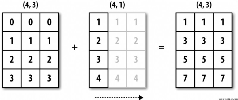
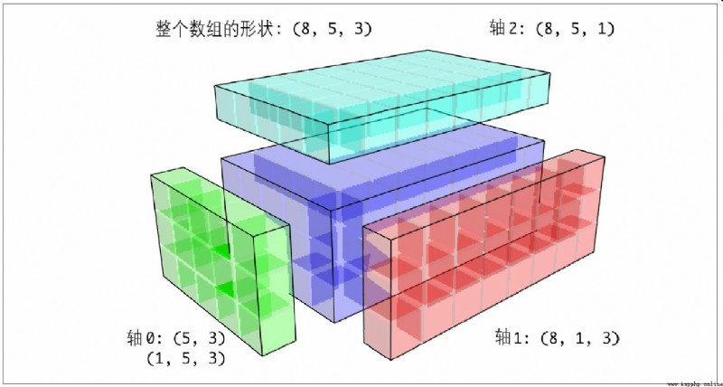
chart A-6 Shows another case , This time it's on a three-dimensional array 0 Axial plus a two-dimensional array .
The broadcast of high-dimensional arrays seems more difficult to understand , In fact, it also follows the broadcasting principle . If not , You will get the following error :
In [93]: arr - arr.mean(1)
---------------------------------------------------------------------------
ValueError Traceback (most recent call last)
<ipython-input-93-7b87b85a20b2> in <module>()
----> 1 arr - arr.mean(1)
ValueError: operands could not be broadcast together with shapes (4,3) (4,)
People often need to divide the lower dimensional array by the arithmetic operation 0 The other axis other than the axis is broadcast upwards . According to the principles of broadcasting , Of smaller arrays “ Broadcast dimension ” It has to be for 1. In the above example of line spacing flattening , This means changing the shape of the row average to (4,1) instead of (4,):
In [94]: arr - arr.mean(1).reshape((4, 1))
Out[94]:
array([[-0.2095, 1.1334, -0.9239],
[ 0.8562, -0.6828, -0.1734],
[-0.3386, 1.0823, -0.7438],
[ 0.3234, -0.8599, 0.5365]])
For the three-dimensional case , Broadcasting on any one dimension in three dimensions is actually reshaping the data into compatible shapes . chart A-7 It describes the shape requirements to be broadcast on each dimension of the 3D array .
So there is a very common problem ( Especially in general algorithms ), That is, a length of... Is added specifically for broadcasting 1 New axis for . although reshape It's a way , But the insertion axis needs to construct a tuple representing the new shape . This is a very depressing process . therefore ,NumPy Arrays provide a special syntax for inserting axes through an indexing mechanism . The following code uses a special np.newaxis Properties and “ whole ” Slice to insert a new axis :
In [95]: arr = np.zeros((4, 4))
In [96]: arr_3d = arr[:, np.newaxis, :]
In [97]: arr_3d.shape
Out[97]: (4, 1, 4)
In [98]: arr_1d = np.random.normal(size=3)
In [99]: arr_1d[:, np.newaxis]
Out[99]:
array([[-2.3594],
[-0.1995],
[-1.542 ]])
In [100]: arr_1d[np.newaxis, :]
Out[100]: array([[-2.3594, -0.1995, -1.542 ]])
therefore , If we have a three-dimensional array , And hope to align the shaft 2 Perform leveling , Then you just need to write the following code :
In [101]: arr = np.random.randn(3, 4, 5)
In [102]: depth_means = arr.mean(2)
In [103]: depth_means
Out[103]:
array([[-0.4735, 0.3971, -0.0228, 0.2001],
[-0.3521, -0.281 , -0.071 , -0.1586],
[ 0.6245, 0.6047, 0.4396, -0.2846]])
In [104]: depth_means.shape
Out[104]: (3, 4)
In [105]: demeaned = arr - depth_means[:, :, np.newaxis]
In [106]: demeaned.mean(2)
Out[106]:
array([[ 0., 0., -0., -0.],
[ 0., 0., -0., 0.],
[ 0., 0., -0., -0.]])
Some readers may think , When flattening a specified axis , Is there a way to be universal without sacrificing performance ? In fact, there are , But it requires some indexing skills :
def demean_axis(arr, axis=0):
means = arr.mean(axis)
# This generalizes things like [:, :, np.newaxis] to N dimensions
indexer = [slice(None)] * arr.ndim
indexer[axis] = np.newaxis
return arr - means[indexer]
The broadcast principle followed by arithmetic operations also applies to the operation of setting array values through the index mechanism . For the simplest case , We can do that :
In [107]: arr = np.zeros((4, 3))
In [108]: arr[:] = 5
In [109]: arr
Out[109]:
array([[ 5., 5., 5.],
[ 5., 5., 5.],
[ 5., 5., 5.],
[ 5., 5., 5.]])
however , Suppose we want to use a one-dimensional array to set the columns of the target array , As long as the shape is compatible :
In [110]: col = np.array([1.28, -0.42, 0.44, 1.6])
In [111]: arr[:] = col[:, np.newaxis]
In [112]: arr
Out[112]:
array([[ 1.28, 1.28, 1.28],
[-0.42, -0.42, -0.42],
[ 0.44, 0.44, 0.44],
[ 1.6 , 1.6 , 1.6 ]])
In [113]: arr[:2] = [[-1.37], [0.509]]
In [114]: arr
Out[114]:
array([[-1.37 , -1.37 , -1.37 ],
[ 0.509, 0.509, 0.509],
[ 0.44 , 0.44 , 0.44 ],
[ 1.6 , 1.6 , 1.6 ]])
Though many NumPy Users will only use the fast element level operations provided by general-purpose functions , But general-purpose functions actually have some advanced uses that allow us to write more concise code without loops .
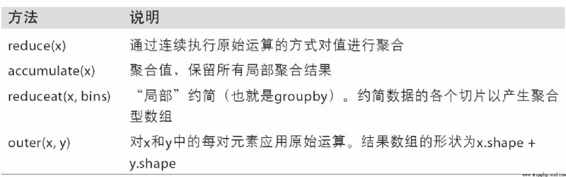
NumPy Each binary of ufunc There are special methods for performing specific vectorization operations . surface A-2 These methods are summarized , I will illustrate them with a few specific examples below .
reduce Accept an array parameter , And through a series of binary operations to aggregate its values ( The axial direction can be indicated ). for example , We can use np.add.reduce Sum the elements in the array :
In [115]: arr = np.arange(10)
In [116]: np.add.reduce(arr)
Out[116]: 45
In [117]: arr.sum()
Out[117]: 45
The starting value depends on ufunc( about add The situation of , Namely 0). If the shaft number is set , The reduction operation will be performed along this axis . This allows you to get answers to certain questions in a more concise way . In the following example , We use it np.logical_and Check whether the values in each row of the array are ordered :
In [118]: np.random.seed(12346) # for reproducibility
In [119]: arr = np.random.randn(5, 5)
In [120]: arr[::2].sort(1) # sort a few rows
In [121]: arr[:, :-1] < arr[:, 1:]
Out[121]:
array([[ True, True, True, True],
[False, True, False, False],
[ True, True, True, True],
[ True, False, True, True],
[ True, True, True, True]], dtype=bool)
In [122]: np.logical_and.reduce(arr[:, :-1] < arr[:, 1:], axis=1)
Out[122]: array([ True, False, True, False, True], dtype=bool)
Be careful ,logical_and.reduce Follow all Methods are equivalent .
ccumulate Follow reduce The relationship is like cumsum Follow sum It's like that . It produces an intermediate with the same size as the original array “ Cumulative ” An array of values :
In [123]: arr = np.arange(15).reshape((3, 5))
In [124]: np.add.accumulate(arr, axis=1)
Out[124]:
array([[ 0, 1, 3, 6, 10],
[ 5, 11, 18, 26, 35],
[10, 21, 33, 46, 60]])
outer Used to calculate the cross product of two arrays :
In [125]: arr = np.arange(3).repeat([1, 2, 2])
In [126]: arr
Out[126]: array([0, 1, 1, 2, 2])
In [127]: np.multiply.outer(arr, np.arange(5))
Out[127]:
array([[0, 0, 0, 0, 0],
[0, 1, 2, 3, 4],
[0, 1, 2, 3, 4],
[0, 2, 4, 6, 8],
[0, 2, 4, 6, 8]])
outer The dimension of the output result is the sum of the two dimensions of the input data :
In [128]: x, y = np.random.randn(3, 4), np.random.randn(5)
In [129]: result = np.subtract.outer(x, y)
In [130]: result.shape
Out[130]: (3, 4, 5)
Last method reduceat Used to calculate “ Local reduction ”, In fact, it is a method for aggregating data slices groupby operation . It accepts a set of... That indicate how values are split and aggregated “ Bin boundary ”:
In [131]: arr = np.arange(10)
In [132]: np.add.reduceat(arr, [0, 5, 8])
Out[132]: array([10, 18, 17])
The end result is arr[0:5]、arr[5:8] as well as arr[8:] Reduction performed on . Just like other methods , You can also pass in a axis Parameters :
In [133]: arr = np.multiply.outer(np.arange(4), np.arange(5))
In [134]: arr
Out[134]:
array([[ 0, 0, 0, 0, 0],
[ 0, 1, 2, 3, 4],
[ 0, 2, 4, 6, 8],
[ 0, 3, 6, 9, 12]])
In [135]: np.add.reduceat(arr, [0, 2, 4], axis=1)
Out[135]:
array([[ 0, 0, 0],
[ 1, 5, 4],
[ 2, 10, 8],
[ 3, 15, 12]])
surface A-2 Part of the ufunc Method .
There are many ways you can write your own NumPy ufuncs. The most common is the use of NumPy C API, But it goes beyond the scope of this book . In this section , Let's talk about pure Python ufunc.
numpy.frompyfunc Accept one Python Function and two parameters representing the number of input and output parameters respectively . for example , The following is a simple function that can implement element level addition :
In [136]: def add_elements(x, y):
.....: return x + y
In [137]: add_them = np.frompyfunc(add_elements, 2, 1)
In [138]: add_them(np.arange(8), np.arange(8))
Out[138]: array([0, 2, 4, 6, 8, 10, 12, 14], dtype=object)
use frompyfunc Created functions always return Python An array of objects , This is very inconvenient . Fortunately, , There's another way , namely numpy.vectorize. Although there is no frompyfunc So powerful , But it allows you to specify the output type :
In [139]: add_them = np.vectorize(add_elements, otypes=[np.float64])
In [140]: add_them(np.arange(8), np.arange(8))
Out[140]: array([ 0., 2., 4., 6., 8., 10., 12., 14.])
Although these two functions provide a way to create ufunc Means of type function , But they are very slow , Because they execute once when calculating each element Python Function call , This will be better than NumPy It's based on C Of ufunc A lot slower :
In [141]: arr = np.random.randn(10000)
In [142]: %timeit add_them(arr, arr)
4.12 ms +- 182 us per loop (mean +- std. dev. of 7 runs, 100 loops each)
In [143]: %timeit np.add(arr, arr)
6.89 us +- 504 ns per loop (mean +- std. dev. of 7 runs, 100000 loops each)
Later in this chapter , I'll introduce the use of Numba(http://numba.pydata.org/), Create fast Python ufuncs.
You may have noticed , What we have discussed so far ndarray Both are homogeneous data containers , in other words , In the memory block it represents , Each element occupies the same number of bytes ( According to dtype And decide ). On the face of it , It seems that it cannot be used to represent heterogeneous or tabular data . Structured arrays are a special kind of ndarray, Each of these elements can be seen as C The structure of language (struct, This is it. “ structured ” The origin of ) or SQL Rows with multiple named fields in the table :
In [144]: dtype = [('x', np.float64), ('y', np.int32)]
In [145]: sarr = np.array([(1.5, 6), (np.pi, -2)], dtype=dtype)
In [146]: sarr
Out[146]:
array([( 1.5 , 6), ( 3.1416, -2)],
dtype=[('x', '<f8'), ('y', '<i4')])
Define structured dtype( Please refer to NumPy Online documentation for ) There are many ways . The most typical method is the tuple list , The format of each tuple is (field_name,field_data_type). such , The elements of the array become tuple objects , Each element in this object can be accessed like a dictionary :
In [147]: sarr[0]
Out[147]: ( 1.5, 6)
In [148]: sarr[0]['y']
Out[148]: 6
The field name is saved dtype.names Properties of the . When accessing a field of a structured array , What is returned is the view of the data , So data replication will not occur :
In [149]: sarr['x']
Out[149]: array([ 1.5 , 3.1416])
In defining structured dtype when , You can set another shape ( It can be an integer , It can also be a tuple ):
In [150]: dtype = [('x', np.int64, 3), ('y', np.int32)]
In [151]: arr = np.zeros(4, dtype=dtype)
In [152]: arr
Out[152]:
array([([0, 0, 0], 0), ([0, 0, 0], 0), ([0, 0, 0], 0), ([0, 0, 0], 0)],
dtype=[('x', '<i8', (3,)), ('y', '<i4')])
under these circumstances , Of each record x The field represents a length of 3 Array of :
In [153]: arr[0]['x']
Out[153]: array([0, 0, 0])
such , visit arr[‘x’] You can get a two-dimensional array , Instead of the one-dimensional array in the previous example :
In [154]: arr['x']
Out[154]:
array([[0, 0, 0],
[0, 0, 0],
[0, 0, 0],
[0, 0, 0]])
This allows you to store complex nested structures in memory blocks of a single array . You can also nest dtype, Make more complex structures . Here is a simple example :
In [155]: dtype = [('x', [('a', 'f8'), ('b', 'f4')]), ('y', np.int32)]
In [156]: data = np.array([((1, 2), 5), ((3, 4), 6)], dtype=dtype)
In [157]: data['x']
Out[157]:
array([( 1., 2.), ( 3., 4.)],
dtype=[('a', '<f8'), ('b', '<f4')])
In [158]: data['y']
Out[158]: array([5, 6], dtype=int32)
In [159]: data['x']['a']
Out[159]: array([ 1., 3.])
pandas Of DataFrame This feature is not directly supported , But its hierarchical indexing mechanism is similar to this .
Follow pandas Of DataFrame comparison ,NumPy Is a relatively low-level tool . It can interpret a single memory block as a tabular structure with arbitrarily complex nested columns . Because each element in the array is represented as a fixed number of bytes in memory , So structured arrays can provide very fast and efficient disk data reading and writing ( Including memory images )、 Network transmission and other functions .
Another common use of structured arrays is , Write the data file as a fixed length record byte stream , This is a C and C++ Common data serialization methods in code ( It can be found in many historical systems in the industry ). Just know the format of the file ( The size of the record 、 The order of the elements 、 Number of bytes, data type, etc ), You can use it np.fromfile Read data into memory . This usage is beyond the scope of this book , Just know that .
Follow Python Built in list ,ndarray Of sort Instance methods are also sorted in place . in other words , Rearranging the contents of an array does not produce a new array :
In [160]: arr = np.random.randn(6)
In [161]: arr.sort()
In [162]: arr
Out[162]: array([-1.082 , 0.3759, 0.8014, 1.1397, 1.2888, 1.8413])
One thing to note when sorting arrays in place , If the target array is just a view , The original array will be modified :
In [163]: arr = np.random.randn(3, 5)
In [164]: arr
Out[164]:
array([[-0.3318, -1.4711, 0.8705, -0.0847, -1.1329],
[-1.0111, -0.3436, 2.1714, 0.1234, -0.0189],
[ 0.1773, 0.7424, 0.8548, 1.038 , -0.329 ]])
In [165]: arr[:, 0].sort() # Sort first column values in-place
In [166]: arr
Out[166]:
array([[-1.0111, -1.4711, 0.8705, -0.0847, -1.1329],
[-0.3318, -0.3436, 2.1714, 0.1234, -0.0189],
[ 0.1773, 0.7424, 0.8548, 1.038 , -0.329 ]])
contrary ,numpy.sort Creates a sorted copy of the original array . in addition , The parameters it accepts ( such as kind) Follow ndarray.sort equally :
In [167]: arr = np.random.randn(5)
In [168]: arr
Out[168]: array([-1.1181, -0.2415, -2.0051, 0.7379, -1.0614])
In [169]: np.sort(arr)
Out[169]: array([-2.0051, -1.1181, -1.0614, -0.2415, 0.7379])
In [170]: arr
Out[170]: array([-1.1181, -0.2415, -2.0051, 0.7379, -1.0614])
Both sorting methods can accept one axis Parameters , To sort the block data separately along the specified axis :
In [171]: arr = np.random.randn(3, 5)
In [172]: arr
Out[172]:
array([[ 0.5955, -0.2682, 1.3389, -0.1872, 0.9111],
[-0.3215, 1.0054, -0.5168, 1.1925, -0.1989],
[ 0.3969, -1.7638, 0.6071, -0.2222, -0.2171]])
In [173]: arr.sort(axis=1)
In [174]: arr
Out[174]:
array([[-0.2682, -0.1872, 0.5955, 0.9111, 1.3389],
[-0.5168, -0.3215, -0.1989, 1.0054, 1.1925],
[-1.7638, -0.2222, -0.2171, 0.3969, 0.6071]])
You may have noticed , Neither of these sorting methods can be set to descending . It doesn't matter , Because array slicing produces views ( in other words , No copies will be produced , Nor does it require any other computational work ). many Python Users are familiar with a little trick about lists :values[::-1] You can return a list in reverse order . Yes ndarray So it is with :
In [175]: arr[:, ::-1]
Out[175]:
array([[ 1.3389, 0.9111, 0.5955, -0.1872, -0.2682],
[ 1.1925, 1.0054, -0.1989, -0.3215, -0.5168],
[ 0.6071, 0.3969, -0.2171, -0.2222, -1.7638]])
In data analysis , It is often necessary to sort data sets according to one or more keys . for example , A data table of student information may need to be sorted by last name and first name ( Last name before first name ). This is an example of an indirect sort , If you have read about pandas Chapter of , I have seen many advanced examples . Given one or more keys , You can get an indexed array of integers ( I affectionately call it an indexer ), The index value indicates the position of the data in the new order .argsort and numpy.lexsort Are the two main ways to achieve this function . Here is a simple example :
In [176]: values = np.array([5, 0, 1, 3, 2])
In [177]: indexer = values.argsort()
In [178]: indexer
Out[178]: array([1, 2, 4, 3, 0])
In [179]: values[indexer]
Out[179]: array([0, 1, 2, 3, 5])
A more complex example , The following code sorts the array according to its first line :
In [180]: arr = np.random.randn(3, 5)
In [181]: arr[0] = values
In [182]: arr
Out[182]:
array([[ 5. , 0. , 1. , 3. , 2. ],
[-0.3636, -0.1378, 2.1777, -0.4728, 0.8356],
[-0.2089, 0.2316, 0.728 , -1.3918, 1.9956]])
In [183]: arr[:, arr[0].argsort()]
Out[183]:
array([[ 0. , 1. , 2. , 3. , 5. ],
[-0.1378, 2.1777, 0.8356, -0.4728, -0.3636],
[ 0.2316, 0.728 , 1.9956, -1.3918, -0.2089]])
lexsort Follow argsort almost , However, it can perform indirect sorting on multiple key arrays at one time ( Dictionary order ). Suppose we want to sort some data identified by last name and first name :
In [184]: first_name = np.array(['Bob', 'Jane', 'Steve', 'Bill', 'Barbara'])
In [185]: last_name = np.array(['Jones', 'Arnold', 'Arnold', 'Jones', 'Walters'])
In [186]: sorter = np.lexsort((first_name, last_name))
In [187]: sorter
Out[187]: array([1, 2, 3, 0, 4])
In [188]: zip(last_name[sorter], first_name[sorter])
Out[188]: <zip at 0x7fa203eda1c8>
Just beginning to use lexsort It may be easier to get dizzy , This is because the order in which the keys are applied is calculated from the last one passed in . It's not hard to see. ,last_name Before first_name Applied .
note :Series and DataFrame Of sort_index as well as Series Of order The method is through variations of these functions ( They must also consider missing values ) Realized .
The stability of the (stable) The sorting algorithm keeps the relative positions of the equivalent elements . For those indirect orders where the relative position has practical significance , This is very important :
In [189]: values = np.array(['2:first', '2:second', '1:first', '1:second',
.....: '1:third'])
In [190]: key = np.array([2, 2, 1, 1, 1])
In [191]: indexer = key.argsort(kind='mergesort')
In [192]: indexer
Out[192]: array([2, 3, 4, 0, 1])
In [193]: values.take(indexer)
Out[193]:
array(['1:first', '1:second', '1:third', '2:first', '2:second'],
dtype='<U8')
mergesort( Merge sort ) Is the only stable sort , It promises to have O(n log n) Performance of ( Spatial complexity ), But its average performance is better than the default quicksort( Quick sort ) Want difference . surface A-3 The available sorting algorithms and their related performance indicators are listed . Most users don't need to know these things at all , But it's always good to know .

One of the purposes of sorting may be to determine the largest or smallest element in the array .NumPy There are two optimization methods ,numpy.partition and np.argpartition, In the first k An array divided by the smallest elements :
In [194]: np.random.seed(12345)
In [195]: arr = np.random.randn(20)
In [196]: arr
Out[196]:
array([-0.2047, 0.4789, -0.5194, -0.5557, 1.9658, 1.3934, 0.0929,
0.2817, 0.769 , 1.2464, 1.0072, -1.2962, 0.275 , 0.2289,
1.3529, 0.8864, -2.0016, -0.3718, 1.669 , -0.4386])
In [197]: np.partition(arr, 3)
Out[197]:
array([-2.0016, -1.2962, -0.5557, -0.5194, -0.3718, -0.4386, -0.2047,
0.2817, 0.769 , 0.4789, 1.0072, 0.0929, 0.275 , 0.2289,
1.3529, 0.8864, 1.3934, 1.9658, 1.669 , 1.2464])
When you call partition(arr, 3), The first three elements in the result are the smallest , There is no specific order .numpy.argpartition And numpy.argsort be similar , Will return the index , Rearrange data to an equivalent order :
In [198]: indices = np.argpartition(arr, 3)
In [199]: indices
Out[199]:
array([16, 11, 3, 2, 17, 19, 0, 7, 8, 1, 10, 6, 12, 13, 14, 15, 5,
4, 18, 9])
In [200]: arr.take(indices)
Out[200]:
array([-2.0016, -1.2962, -0.5557, -0.5194, -0.3718, -0.4386, -0.2047,
0.2817, 0.769 , 0.4789, 1.0072, 0.0929, 0.275 , 0.2289,
1.3529, 0.8864, 1.3934, 1.9658, 1.669 , 1.2464])
searchsorted Is an array method that performs binary lookup on an ordered array , As long as the value is inserted into the position it returns, the order of the array can be maintained :
In [201]: arr = np.array([0, 1, 7, 12, 15])
In [202]: arr.searchsorted(9)
Out[202]: 3
You can pass in a set of values to get a set of indexes :
In [203]: arr.searchsorted([0, 8, 11, 16])
Out[203]: array([0, 3, 3, 5])
As can be seen from the above results , For elements 0,searchsorted Returns the 0. This is because its default behavior is to return the left index of the group of equal values :
In [204]: arr = np.array([0, 0, 0, 1, 1, 1, 1])
In [205]: arr.searchsorted([0, 1])
Out[205]: array([0, 3])
In [206]: arr.searchsorted([0, 1], side='right')
Out[206]: array([3, 7])
Look again. searchsorted Another use of , Suppose we have an array of data ( Where the value is in 0 To 10000 Between ), There is another expression “ Bin boundary ” Array of , We want to use it to split the data array :
In [207]: data = np.floor(np.random.uniform(0, 10000, size=50))
In [208]: bins = np.array([0, 100, 1000, 5000, 10000])
In [209]: data
Out[209]:
array([ 9940., 6768., 7908., 1709., 268., 8003., 9037., 246.,
4917., 5262., 5963., 519., 8950., 7282., 8183., 5002.,
8101., 959., 2189., 2587., 4681., 4593., 7095., 1780.,
5314., 1677., 7688., 9281., 6094., 1501., 4896., 3773.,
8486., 9110., 3838., 3154., 5683., 1878., 1258., 6875.,
7996., 5735., 9732., 6340., 8884., 4954., 3516., 7142.,
5039., 2256.])
then , To get the number of the interval to which each data point belongs ( among 1 Represents a bin [0,100)), We can use it directly searchsorted:
In [210]: labels = bins.searchsorted(data)
In [211]: labels
Out[211]:
array([4, 4, 4, 3, 2, 4, 4, 2, 3, 4, 4, 2, 4, 4, 4, 4, 4, 2, 3, 3, 3, 3, 4,
3, 4, 3, 4, 4, 4, 3, 3, 3, 4, 4, 3, 3, 4, 3, 3, 4, 4, 4, 4, 4, 4, 3,
3, 4, 4, 3])
adopt pandas Of groupby Using this result, the original data set can be easily split :
In [212]: pd.Series(data).groupby(labels).mean()
Out[212]:
2 498.000000
3 3064.277778
4 7389.035714
dtype: float64
#A.7 use Numba Write fast NumPy function
Numba It's an open source project , It can take advantage of CPUs、GPUs Or similar hardware NumPy Data to create a quick function . It has been used. LLVM project (http://llvm.org/), take Python Code to machine code .
To introduce Numba, Consider a pure Python function , It USES for Loop evaluation expression (x - y).mean():
import numpy as np
def mean_distance(x, y):
nx = len(x)
result = 0.0
count = 0
for i in range(nx):
result += x[i] - y[i]
count += 1
return result / count
This function is very slow :
In [209]: x = np.random.randn(10000000)
In [210]: y = np.random.randn(10000000)
In [211]: %timeit mean_distance(x, y)
1 loop, best of 3: 2 s per loop
In [212]: %timeit (x - y).mean()
100 loops, best of 3: 14.7 ms per loop
NumPy The version of is faster than it 100 times . We can convert this function to compiled Numba function , Use numba.jit function :
In [213]: import numba as nb
In [214]: numba_mean_distance = nb.jit(mean_distance)
It can also be written as a decorator :
@nb.jit
def mean_distance(x, y):
nx = len(x)
result = 0.0
count = 0
for i in range(nx):
result += x[i] - y[i]
count += 1
return result / count
It's better than vectorized NumPy fast :
In [215]: %timeit numba_mean_distance(x, y)
100 loops, best of 3: 10.3 ms per loop
Numba Can't compile Python Code , But it supports pure Python Write a part of , You can write numerical algorithms .
Numba Is a deep Library , Support a variety of hardware 、 Compile mode and user plug-ins . It can also compile NumPy Python API Part of , without for loop .Numba You can also identify structures that can be encoded as machines , But if you call CPython API, It doesn't know how to compile .Numba Of jit The function has an option ,nopython=True, It limits the ability to be converted to Python The code of the code , This code can be compiled into LLVM, But nothing Python C API call .jit(nopython=True) There is a short alias numba.njit.
The previous example , We can also write like this :
from numba import float64, njit
@njit(float64(float64[:], float64[:]))
def mean_distance(x, y):
return (x - y).mean()
I suggest you study Numba Online documentation for (http://numba.pydata.org/). The next section describes how to create a custom Numpy ufunc Examples of objects .
numba.vectorize Created a compiled NumPy ufunc, It works with the built-in ufunc It's like . Consider one numpy.add Of Python Example :
from numba import vectorize
@vectorize
def nb_add(x, y):
return x + y
Now there is :
In [13]: x = np.arange(10)
In [14]: nb_add(x, x)
Out[14]: array([ 0., 2., 4., 6., 8., 10., 12., 14., 16., 18.])
In [15]: nb_add.accumulate(x, 0)
Out[15]: array([ 0., 1., 3., 6., 10., 15., 21., 28., 36., 45.])
I'm at number one 4 It's mentioned in the chapter ,np.save and np.load It can be used to read and write arrays stored in binary format on disk . There are also tools available for more complex scenarios . Especially memory images (memory map), It allows you to handle data sets that are not in memory .
Memory image file is a way to treat very large binary data files on disk as arrays in memory .NumPy A similar to ndarray Of memmap object , It allows large files to be read and written in small segments , Instead of reading the entire array into memory at once . in addition ,memmap It also has the same method as an ordinary array , therefore , Basically as long as it can be used for ndarray Our algorithm can also be used for memmap.
To create a memory image , You can use functions np.memmap And pass in a file path 、 data type 、 Shape and file mode :
In [214]: mmap = np.memmap('mymmap', dtype='float64', mode='w+',
.....: shape=(10000, 10000))
In [215]: mmap
Out[215]:
memmap([[ 0., 0., 0., ..., 0., 0., 0.],
[ 0., 0., 0., ..., 0., 0., 0.],
[ 0., 0., 0., ..., 0., 0., 0.],
...,
[ 0., 0., 0., ..., 0., 0., 0.],
[ 0., 0., 0., ..., 0., 0., 0.],
[ 0., 0., 0., ..., 0., 0., 0.]])
Yes memmap Slicing will return a view of the data on disk :
In [216]: section = mmap[:5]
If you assign data to these views : The data will be cached in memory first ( like Python The file object of ), call flush You can write it to disk :
In [217]: section[:] = np.random.randn(5, 10000)
In [218]: mmap.flush()
In [219]: mmap
Out[219]:
memmap([[ 0.7584, -0.6605, 0.8626, ..., 0.6046, -0.6212, 2.0542],
[-1.2113, -1.0375, 0.7093, ..., -1.4117, -0.1719, -0.8957],
[-0.1419, -0.3375, 0.4329, ..., 1.2914, -0.752 , -0.44 ],
...,
[ 0. , 0. , 0. , ..., 0. , 0. , 0. ],
[ 0. , 0. , 0. , ..., 0. , 0. , 0. ],
[ 0. , 0. , 0. , ..., 0. , 0. , 0. ]])
In [220]: del mmap
As long as a memory image is out of scope , It will be recycled by the garbage collector , Any previous changes to it will be written to disk . When opening an existing memory image , You still need to specify the data type and shape , Because the file on the disk is just a piece of binary data , No metadata :
In [221]: mmap = np.memmap('mymmap', dtype='float64', shape=(10000, 10000))
In [222]: mmap
Out[222]:
memmap([[ 0.7584, -0.6605, 0.8626, ..., 0.6046, -0.6212, 2.0542],
[-1.2113, -1.0375, 0.7093, ..., -1.4117, -0.1719, -0.8957],
[-0.1419, -0.3375, 0.4329, ..., 1.2914, -0.752 , -0.44 ],
...,
[ 0. , 0. , 0. , ..., 0. , 0. , 0. ],
[ 0. , 0. , 0. , ..., 0. , 0. , 0. ],
[ 0. , 0. , 0. , ..., 0. , 0. , 0. ]])
Memory images can be structured or nested as described earlier dtype.
PyTables and h5py these two items. Python The project can be NumPy The storage of array data is efficient and compressible HDF5 Format (HDF intend “ Hierarchical data format ”). You can safely put hundreds of GB even to the extent that TB Data stored as HDF5 Format . To learn Python Use HDF5, Please refer to pandas Online document .
Use NumPy The performance of the code is generally very good , Because array operations are generally better than pure Python The cycle is much faster . Here's a rough list of things to note :
If used alone NumPy In any case, the required performance index can not be reached , You can consider using C、Fortran or Cython( I'll give you a brief introduction later ) To write code . I often use it in my work Cython(http://cython.org), Because it doesn't cost me too much energy to get C Language like performance .
Although this topic is a little beyond the scope of this book , But I still want to mention , Because in some application scenarios , The memory layout of the array can have a great impact on the computing speed . This is because the performance difference is similar to CPU The cache of (cache) System related . Accessing contiguous memory blocks during operations ( for example , To C Row sum of sequentially stored arrays ) Usually the fastest , Because the memory subsystem will cache the appropriate memory blocks to the super high speed L1 or L2CPU Cache in . Besides ,NumPy Of C Basic language code ( some ) Optimized for continuous storage , In this way, some leapfrog memory access can be avoided .
The memory layout of an array is continuous , That is, the elements are in the order they appear in the array ( namely Fortran type ( Column priority ) or C type ( Line first )) Stored in memory . By default ,NumPy Array is based on C Created in a continuous way . Column first array ( such as C Transpose of continuous array of type ) Also known as Fortran Type continuous . adopt ndarray Of flags Property to view this information :
In [225]: arr_c = np.ones((1000, 1000), order='C')
In [226]: arr_f = np.ones((1000, 1000), order='F')
In [227]: arr_c.flags
Out[227]:
C_CONTIGUOUS : True
F_CONTIGUOUS : False
OWNDATA : True
WRITEABLE : True
ALIGNED : True
UPDATEIFCOPY : False
In [228]: arr_f.flags
Out[228]:
C_CONTIGUOUS : False
F_CONTIGUOUS : True
OWNDATA : True
WRITEABLE : True
ALIGNED : True
UPDATEIFCOPY : False
In [229]: arr_f.flags.f_contiguous
Out[229]: True
In this case , Sum the rows of two arrays , In theory, ,arr_c than arr_f fast , because arr_c The rows of are contiguous in memory . We can do it in IPython of use %timeit Let's make sure :
In [230]: %timeit arr_c.sum(1)
784 us +- 10.4 us per loop (mean +- std. dev. of 7 runs, 1000 loops each)
In [231]: %timeit arr_f.sum(1)
934 us +- 29 us per loop (mean +- std. dev. of 7 runs, 1000 loops each)
If you want to go from NumPy To improve performance , This should be the place to start . If the memory order of the array does not meet your requirements , Use copy And pass in ’C’ or ’F’ To solve the problem :
In [232]: arr_f.copy('C').flags
Out[232]:
C_CONTIGUOUS : True
F_CONTIGUOUS : False
OWNDATA : True
WRITEABLE : True
ALIGNED : True
UPDATEIFCOPY : False
Be careful , When constructing the view of an array , The results are not necessarily continuous :
In [233]: arr_c[:50].flags.contiguous
Out[233]: True
In [234]: arr_c[:, :50].flags
Out[234]:
C_CONTIGUOUS : False
F_CONTIGUOUS : False
OWNDATA : False
WRITEABLE : True
ALIGNED : True
UPDATEIFCOPY : False