Data transferred from (GitHub Address ):https://github.com/wesm/pydata-book Friends in need can go by themselves github download 
The first 2 In the chapter , We learned IPython shell and Jupyter notebook The basis of . In this chapter , We will explore IPython Deeper functions , From the console or in jupyter Use .
Ipython Maintains a small database on disk , Used to save each instruction executed . Its uses are :
These functions are shell in , than notebook More useful , because notebook The design is to put the input and output code into each code grid .
Ipython It allows you to search and execute previous code or other commands . This function is very useful , Because you may need to repeat the same command , for example %run command , Or other codes . Suppose you have to perform :
In[7]: %run first/second/third/data_script.py
The successful running , Then check the results , It is found that the calculation is wrong . Solve the problem , And then modified data_script.py, You can enter some %run command , Then press Ctrl+P Or up arrow . This allows you to search for historical commands , Commands that match input characters . Multiple press Ctrl+P Or up arrow , Will continue to search for commands . If you want to execute the command you want to execute , Don't be scared . You can press Ctrl-N Or down arrow , Move history command forward . After doing this several times , You can press these keys without thinking !
Ctrl-R Can bring about as Unix style shell( such as bash shell) Of readline Some incremental search functions of . stay Windows On ,readline The function is to be IPython Imitative . Use this feature , According to the first Ctrl-R, Then enter some characters you want to search contained in the input line :
In [1]: a_command = foo(x, y, z)
(reverse-i-search)`com': a_command = foo(x, y, z)
Ctrl-R Will cycle through history , Find every line of matching characters .
Forgetting to assign the result of a function call to a variable is annoying .IPython One of the session In a special variable , Store inputs and outputs Python References to objects . The first two outputs are stored in _( An underline ) and __( Two underscores ) Variable :
In [24]: 2 ** 27
Out[24]: 134217728
In [25]: _
Out[25]: 134217728
Input variables are stored in names similar to _iX Variables in ,X Is the number of the input line . For each input variable , There is a corresponding output variable _X. Therefore, in the input page 27 After line , There will be two new variables _27 ( Output ) and _i27( Input ):
In [26]: foo = 'bar'
In [27]: foo
Out[27]: 'bar'
In [28]: _i27
Out[28]: u'foo'
In [29]: _27
Out[29]: 'bar'
Because the input variable is a string , They can use Python Of exec Keyword execute again :
In [30]: exec(_i27)
here ,_i27 Is in In [27] Input code .
There are several magic functions that allow you to use input and output history .%hist You can print all or part of the input history , With or without a number .%reset You can clean up the interaction namespace , Or input and output caching .%xdel Magic functions can remove IPython All references to a particular object in . For more on these magic methods , Please view the document .
Warning : When dealing with very large data sets , Remember IPython The history of input and output of will cause the referenced object not to be garbage collected ( Free memory ), Even if you use del Keyword to delete a variable from the interaction namespace . under these circumstances , Careful use xdel % and %reset It can help you avoid getting into memory problems .
IPython Another feature of is the seamless connection between the file system and the operating system . It means , While doing other things at the same time , No need to quit IPython, It can be like Windows or Unix Use the command line , Include shell command 、 Change directory 、 use Python object ( List or string ) Store results . It also has simple command aliases and directory Bookmarks .
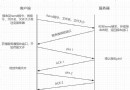
surface B-1 Summarizes the call shell Magic functions and syntax of commands . I will introduce these functions in the following sections .
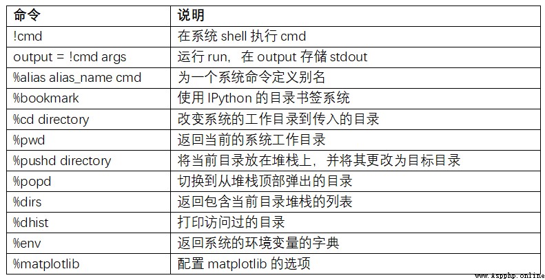
Start a line with an exclamation point , Is to tell IPython Execute everything after the exclamation point . This means that you can delete files ( It depends on the operating system , use rm or del)、 Change directory or execute any other command .
By adding an exclamation point to the variable , You can store the console output of a command in a variable . for example , On my internet based Linux On a host of , I can get IP The address is Python Variable :
In [1]: ip_info = !ifconfig wlan0 | grep "inet "
In [2]: ip_info[0].strip()
Out[2]: 'inet addr:10.0.0.11 Bcast:10.0.0.255 Mask:255.255.255.0'
Back to Python object ip_info It is actually a custom list type , It contains multiple versions of console output .
When using !,IPython You can also replace the... Defined in the current environment Python value . To do this , You can prefix the variable name with $ Symbol :
In [3]: foo = 'test*'
In [4]: !ls $foo
test4.py test.py test.xml
%alias Magic functions can be customized shell Shortcut to command . Take a simple example :
In [1]: %alias ll ls -l
In [2]: ll /usr
total 332
drwxr-xr-x 2 root root 69632 2012-01-29 20:36 bin/
drwxr-xr-x 2 root root 4096 2010-08-23 12:05 games/
drwxr-xr-x 123 root root 20480 2011-12-26 18:08 include/
drwxr-xr-x 265 root root 126976 2012-01-29 20:36 lib/
drwxr-xr-x 44 root root 69632 2011-12-26 18:08 lib32/
lrwxrwxrwx 1 root root 3 2010-08-23 16:02 lib64 -> lib/
drwxr-xr-x 15 root root 4096 2011-10-13 19:03 local/
drwxr-xr-x 2 root root 12288 2012-01-12 09:32 sbin/
drwxr-xr-x 387 root root 12288 2011-11-04 22:53 share/
drwxrwsr-x 24 root src 4096 2011-07-17 18:38 src/
You can execute multiple commands , Just like on the command line , Just separate them with semicolons :
In [558]: %alias test_alias (cd examples; ls; cd ..)
In [559]: test_alias
macrodata.csv spx.csv tips.csv
When session end , The alias you defined will be invalid . To create a permanent alias , Configuration is required .
IPython There is a simple directory bookmarking system , Allows you to save aliases for commonly used directories , It will be very convenient to jump around . for example , Suppose you want to create a bookmark , Point to the supplementary contents of this book :
In [6]: %bookmark py4da /home/wesm/code/pydata-book
After doing so , When using %cd Magic command , You can use the defined bookmarks :
In [7]: cd py4da
(bookmark:py4da) -> /home/wesm/code/pydata-book
/home/wesm/code/pydata-book
If the name of the bookmark , Duplicate the name of a directory with the current working directory , You can use -b Sign to override , Where to use bookmarks . Use %bookmark Of -l Options , You can list all bookmarks :
In [8]: %bookmark -l
Current bookmarks:
py4da -> /home/wesm/code/pydata-book-source
Bookmarks , Different from aliases , stay session Between is maintained .
In addition to being an excellent interactive computing and data exploration environment ,IPython It also works Python Software development tools . In data analysis , The most important thing is to have the right code . Fortunately, ,IPython Tightly integrated and enhanced Python Built in pdb The debugger . second , Need fast code . For this point ,IPython There are easy-to-use code timing and analysis tools . I will cover these tools in detail .
IPython Debugger for tab completion 、 Grammar enhancement 、 Line by line exception tracking enhances pdb. The best time to debug code is when an error has just occurred . After the exception occurs, enter %debug, The debugger starts , Go to the stack frame where the exception is thrown :
In [2]: run examples/ipython_bug.py
---------------------------------------------------------------------------
AssertionError Traceback (most recent call last)
/home/wesm/code/pydata-book/examples/ipython_bug.py in <module>()
13 throws_an_exception()
14
---> 15 calling_things()
/home/wesm/code/pydata-book/examples/ipython_bug.py in calling_things()
11 def calling_things():
12 works_fine()
---> 13 throws_an_exception()
14
15 calling_things()
/home/wesm/code/pydata-book/examples/ipython_bug.py in throws_an_exception()
7 a = 5
8 b = 6
----> 9 assert(a + b == 10)
10
11 def calling_things():
AssertionError:
In [3]: %debug
> /home/wesm/code/pydata-book/examples/ipython_bug.py(9)throws_an_exception()
8 b = 6
----> 9 assert(a + b == 10)
10
ipdb>
Once in the debugger , You can perform any Python Code , Check all objects and data in each stack frame ( The interpreter keeps them active ). The default is to start at the lowest level of error occurrence . adopt u(up) and d(down), You can switch between stack traces at different levels :
ipdb> u
> /home/wesm/code/pydata-book/examples/ipython_bug.py(13)calling_things()
12 works_fine()
---> 13 throws_an_exception()
14
perform %pdb command , You can let... When any exception occurs IPython Automatically start the debugger , Many users will find this feature very easy to use .
It's also easy to help develop code with a debugger , Especially if you want to set breakpoints or move between functions and scripts , To check the status of each phase . There are many ways to achieve . The first is to use %run and -d, It calls the debugger before executing any code passed in to the script . You must press at once s(step) To enter the script :
In [5]: run -d examples/ipython_bug.py
Breakpoint 1 at /home/wesm/code/pydata-book/examples/ipython_bug.py:1
NOTE: Enter 'c' at the ipdb> prompt to start your script.
> <string>(1)<module>()
ipdb> s
--Call--
> /home/wesm/code/pydata-book/examples/ipython_bug.py(1)<module>()
1---> 1 def works_fine():
2 a = 5
3 b = 6
then , You can decide how to work . for example , The exception in front , We can set a breakpoint , In the call works_fine Before , Then run the script , Press... When a breakpoint is encountered c(continue):
ipdb> b 12
ipdb> c
> /home/wesm/code/pydata-book/examples/ipython_bug.py(12)calling_things()
11 def calling_things():
2--> 12 works_fine()
13 throws_an_exception()
At this time , You can step Get into works_fine(), Or by pressing n(next) perform works_fine(), Go to the next line :
ipdb> n
> /home/wesm/code/pydata-book/examples/ipython_bug.py(13)calling_things()
2 12 works_fine()
---> 13 throws_an_exception()
14
then , We can enter throws_an_exception, Get to the wrong line , Check the variable . Be careful , Debugger commands are preceded by variable names , Add an exclamation point before the variable name ! You can view the content :
ipdb> s
--Call--
> /home/wesm/code/pydata-book/examples/ipython_bug.py(6)throws_an_exception()
5
----> 6 def throws_an_exception():
7 a = 5
ipdb> n
> /home/wesm/code/pydata-book/examples/ipython_bug.py(7)throws_an_exception()
6 def throws_an_exception():
----> 7 a = 5
8 b = 6
ipdb> n
> /home/wesm/code/pydata-book/examples/ipython_bug.py(8)throws_an_exception()
7 a = 5
----> 8 b = 6
9 assert(a + b == 10)
ipdb> n
> /home/wesm/code/pydata-book/examples/ipython_bug.py(9)throws_an_exception()
8 b = 6
----> 9 assert(a + b == 10)
10
ipdb> !a
5
ipdb> !b
6
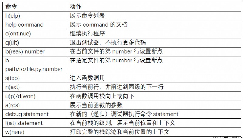
Improving your proficiency with the interactive debugger requires practice and experience . surface B-2, Lists all debugger commands . If you get used to IDE, You may feel that the terminal debugger will not work well at the beginning , But I will feel better and better . some Python Of IDEs There are good ones GUI The debugger , Just choose the one that is easy to handle .
There are other things you can do with the debugger . The first is to use a special set_trace function ( according to pdb.set_trace Named ), This is a simple breakpoint . There are two other ways you might want to use ( Like me , Add it to IPython Configuration of ):
from IPython.core.debugger import Pdb
def set_trace():
Pdb(color_scheme='Linux').set_trace(sys._getframe().f_back)
def debug(f, *args, **kwargs):
pdb = Pdb(color_scheme='Linux')
return pdb.runcall(f, *args, **kwargs)
The first function set_trace It's simple . If you want to stop for a while and go over it ( For example, before an exception occurs ), Can be used anywhere in the code set_trace:
In [7]: run examples/ipython_bug.py
> /home/wesm/code/pydata-book/examples/ipython_bug.py(16)calling_things()
15 set_trace()
---> 16 throws_an_exception()
17
Press c(continue) You can keep the code moving normally .
We just saw debug function , You can easily use the debugger when calling any function . Suppose we write the following function , Want to analyze its logic step by step :
def f(x, y, z=1):
tmp = x + y
return tmp / z
Use generally f, It's like f(1, 2, z=3). And to get in f, take f Pass as the first parameter to debug, Then pass the position and keyword parameters to f:
In [6]: debug(f, 1, 2, z=3)
> <ipython-input>(2)f()
1 def f(x, y, z):
----> 2 tmp = x + y
3 return tmp / z
ipdb>
These two simple methods have saved me a lot of time .
Last , The debugger can work with %run Use it together . The script runs %run -d, You can go directly to the debugger , Set breakpoints and start scripts at will :
In [1]: %run -d examples/ipython_bug.py
Breakpoint 1 at /home/wesm/code/pydata-book/examples/ipython_bug.py:1
NOTE: Enter 'c' at the ipdb> prompt to start your script.
> <string>(1)<module>()
ipdb>
add -b And line number , You can preset a breakpoint :
In [2]: %run -d -b2 examples/ipython_bug.py
Breakpoint 1 at /home/wesm/code/pydata-book/examples/ipython_bug.py:2
NOTE: Enter 'c' at the ipdb> prompt to start your script.
> <string>(1)<module>()
ipdb> c
> /home/wesm/code/pydata-book/examples/ipython_bug.py(2)works_fine()
1 def works_fine():
1---> 2 a = 5
3 b = 6
ipdb>
For large and long-running data analysis applications , You may want to measure the execution time of different components or individual function call statements . You may want to know which function takes the longest time . Fortunately, ,IPython It allows you to develop and test code , This information is easily available .
For manual use time Module and its functions time.clock and time.time Time the code , Monotonous and repetitive , Because I have to write some boring templating code :
import time
start = time.time()
for i in range(iterations):
# some code to run here
elapsed_per = (time.time() - start) / iterations
Because this is a very common operation ,IPython There are two magic functions ,%time and %timeit, Can automate this process .
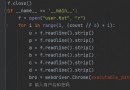
%time Will run the statement once , Report the total execution time . Suppose we have a large list of strings , We want to compare different ways of picking out a particular starting string . Here is one that contains 600000 List of strings , And two ways , To select foo Starting string :
# a very large list of strings
strings = ['foo', 'foobar', 'baz', 'qux',
'python', 'Guido Van Rossum'] * 100000
method1 = [x for x in strings if x.startswith('foo')]
method2 = [x for x in strings if x[:3] == 'foo']
It seems that their performance should be of the same level , But the truth is ? use %time Make a measurement :
In [561]: %time method1 = [x for x in strings if x.startswith('foo')]
CPU times: user 0.19 s, sys: 0.00 s, total: 0.19 s
Wall time: 0.19 s
In [562]: %time method2 = [x for x in strings if x[:3] == 'foo']
CPU times: user 0.09 s, sys: 0.00 s, total: 0.09 s
Wall time: 0.09 s
Wall time(wall-clock time Abbreviation ) Is the main concern . The first method is more than twice the second method , But this measurement method is not accurate . If you use %time Multiple measurements , You will find that the results are variable . To be more accurate , have access to %timeit Magic functions . Give any statement , It can run this statement multiple times to get a more accurate time :
In [563]: %timeit [x for x in strings if x.startswith('foo')]
10 loops, best of 3: 159 ms per loop
In [564]: %timeit [x for x in strings if x[:3] == 'foo']
10 loops, best of 3: 59.3 ms per loop
This example illustrates the understanding of Python Standard library 、NumPy、pandas And other libraries . In large data analysis , These milliseconds will accumulate !
%timeit It is especially suitable for analyzing statements and functions with short execution time , Even microseconds or nanoseconds . These times may seem unimportant , But one 20 Microsecond function execution 1 A million times is better than one 5 Microsecond function length 15 second . In the previous example , We can directly compare two string operations , To understand their performance characteristics :
In [565]: x = 'foobar'
In [566]: y = 'foo'
In [567]: %timeit x.startswith(y)
1000000 loops, best of 3: 267 ns per loop
In [568]: %timeit x[:3] == y
10000000 loops, best of 3: 147 ns per loop
Analyzing code is closely related to code timing , Except that it focuses on “ Where time goes ”.Python The main analysis tool is cProfile modular , It is not limited to IPython.cProfile Will execute a program or any block of code , And it will track the execution time of each function .
Use cProfile The usual way to do this is to run an entire program from the command line , Output the cumulative time of each function . Suppose we have a simple script that performs linear algebraic operations in a loop ( Calculate a series of 100×100 The maximum absolute eigenvalue of a matrix ):
import numpy as np
from numpy.linalg import eigvals
def run_experiment(niter=100):
K = 100
results = []
for _ in xrange(niter):
mat = np.random.randn(K, K)
max_eigenvalue = np.abs(eigvals(mat)).max()
results.append(max_eigenvalue)
return results
some_results = run_experiment()
print 'Largest one we saw: %s' % np.max(some_results)
You can use it. cProfile Run this script , Use the following command line :
python -m cProfile cprof_example.py
After running , You will find that the output is sorted by function name . It's a little hard to see who's spending more time , It is best to -s Specified sorting :
$ python -m cProfile -s cumulative cprof_example.py
Largest one we saw: 11.923204422
15116 function calls (14927 primitive calls) in 0.720 seconds
Ordered by: cumulative time
ncalls tottime percall cumtime percall filename:lineno(function)
1 0.001 0.001 0.721 0.721 cprof_example.py:1(<module>)
100 0.003 0.000 0.586 0.006 linalg.py:702(eigvals)
200 0.572 0.003 0.572 0.003 {
numpy.linalg.lapack_lite.dgeev}
1 0.002 0.002 0.075 0.075 __init__.py:106(<module>)
100 0.059 0.001 0.059 0.001 {
method 'randn')
1 0.000 0.000 0.044 0.044 add_newdocs.py:9(<module>)
2 0.001 0.001 0.037 0.019 __init__.py:1(<module>)
2 0.003 0.002 0.030 0.015 __init__.py:2(<module>)
1 0.000 0.000 0.030 0.030 type_check.py:3(<module>)
1 0.001 0.001 0.021 0.021 __init__.py:15(<module>)
1 0.013 0.013 0.013 0.013 numeric.py:1(<module>)
1 0.000 0.000 0.009 0.009 __init__.py:6(<module>)
1 0.001 0.001 0.008 0.008 __init__.py:45(<module>)
262 0.005 0.000 0.007 0.000 function_base.py:3178(add_newdoc)
100 0.003 0.000 0.005 0.000 linalg.py:162(_assertFinite)
Only the front 15 That's ok . scanning cumtime Column , It's easy to see how much time each function takes . If a function calls another function , Timing doesn't stop .cProfile The start and end times of each function are recorded , Use them for timing .
Except on the command line ,cProfile It can also be used in programs , Analyze arbitrary code blocks , Instead of running a new process .Ipython Of %prun and %run -p, There is a convenient interface to realize this function .%prun Use similar cProfile Command line options for , But you can analyze any Python sentence , Not the whole thing py file :
In [4]: %prun -l 7 -s cumulative run_experiment()
4203 function calls in 0.643 seconds
Ordered by: cumulative time
List reduced from 32 to 7 due to restriction <7>
ncalls tottime percall cumtime percall filename:lineno(function)
1 0.000 0.000 0.643 0.643 <string>:1(<module>)
1 0.001 0.001 0.643 0.643 cprof_example.py:4(run_experiment)
100 0.003 0.000 0.583 0.006 linalg.py:702(eigvals)
200 0.569 0.003 0.569 0.003 {
numpy.linalg.lapack_lite.dgeev}
100 0.058 0.001 0.058 0.001 {
method 'randn'}
100 0.003 0.000 0.005 0.000 linalg.py:162(_assertFinite)
200 0.002 0.000 0.002 0.000 {
method 'all' of 'numpy.ndarray'}
alike , call %run -p -s cumulative cprof_example.py It has the same function as the command line , You just don't have to leave Ipython.
stay Jupyter notebook in , You can use %%prun Magic methods ( Two %) To analyze a whole piece of code . This will bring up a separate window with analysis output . Easy to answer some questions quickly , such as “ Why did this code take so long ”?
Use IPython or Jupyter, There are other tools that can make analysis easier to understand . One of them is SnakeViz(https://github.com/jiffyclub/snakeviz/), It will use d3.js Generate an interactive visual interface for analysis results .
In some cases , use %prun( Or other based on cProfile Analysis method of ) Information obtained , The whole process of not getting the function execution time , Or the result is too complicated , Add the function name , It is difficult to interpret . In this case , There is a small library called line_profiler( Can pass PyPI Or package management tools ). It contains IPython plug-in unit , You can enable a new magic function %lprun, One or more functions can be analyzed line by line . You can modify it IPython To configure ( see IPython Documentation or configuration section later in this chapter ) Join the following line , Enable this plug-in :
# A list of dotted module names of IPython extensions to load.
c.TerminalIPythonApp.extensions = ['line_profiler']
You can also run commands :
%load_ext line_profiler
line_profiler It can also be used in programs ( View the full documentation ), But in IPython Is the most powerful . Suppose you have a module with the following code prof_mod, Do some NumPy Array operation :
from numpy.random import randn
def add_and_sum(x, y):
added = x + y
summed = added.sum(axis=1)
return summed
def call_function():
x = randn(1000, 1000)
y = randn(1000, 1000)
return add_and_sum(x, y)
If you want to know add_and_sum Function performance ,%prun The following can be given :
In [569]: %run prof_mod
In [570]: x = randn(3000, 3000)
In [571]: y = randn(3000, 3000)
In [572]: %prun add_and_sum(x, y)
4 function calls in 0.049 seconds
Ordered by: internal time
ncalls tottime percall cumtime percall filename:lineno(function)
1 0.036 0.036 0.046 0.046 prof_mod.py:3(add_and_sum)
1 0.009 0.009 0.009 0.009 {
method 'sum' of 'numpy.ndarray'}
1 0.003 0.003 0.049 0.049 <string>:1(<module>)
The above method is not very enlightening . Activated IPython plug-in unit line_profiler, New orders %lprun You can use it. . The difference in use is , We have to tell %lprun Which function to analyze . Grammar is :
%lprun -f func1 -f func2 statement_to_profile
We want to analyze add_and_sum, function :
In [573]: %lprun -f add_and_sum add_and_sum(x, y)
Timer unit: 1e-06 s
File: prof_mod.py
Function: add_and_sum at line 3
Total time: 0.045936 s
Line # Hits Time Per Hit % Time Line Contents
==============================================================
3 def add_and_sum(x, y):
4 1 36510 36510.0 79.5 added = x + y
5 1 9425 9425.0 20.5 summed = added.sum(axis=1)
6 1 1 1.0 0.0 return summed
This makes it easy to interpret . We analyzed the same functions as in the code statements . Look at the previous module code , We can call call_function And to it and add_and_sum Analyze , Get a complete code performance summary :
In [574]: %lprun -f add_and_sum -f call_function call_function()
Timer unit: 1e-06 s
File: prof_mod.py
Function: add_and_sum at line 3
Total time: 0.005526 s
Line # Hits Time Per Hit % Time Line Contents
==============================================================
3 def add_and_sum(x, y):
4 1 4375 4375.0 79.2 added = x + y
5 1 1149 1149.0 20.8 summed = added.sum(axis=1)
6 1 2 2.0 0.0 return summed
File: prof_mod.py
Function: call_function at line 8
Total time: 0.121016 s
Line # Hits Time Per Hit % Time Line Contents
==============================================================
8 def call_function():
9 1 57169 57169.0 47.2 x = randn(1000, 1000)
10 1 58304 58304.0 48.2 y = randn(1000, 1000)
11 1 5543 5543.0 4.6 return add_and_sum(x, y)
My experience is to use %prun (cProfile) Conduct macro analysis ,%lprun (line_profiler) Do microscopic analysis . It is best to understand both of these tools .
note : Use %lprun The reason why the function name must be specified is that the execution time of tracking each line is too much . Tracking useless functions can significantly change the results .
Write code quickly and easily 、 Debugging and using is everyone's goal . Besides the code style , Process details ( Such as code overloading ) It also needs some adjustment .
therefore , The content of this section is more like an art than a science , You still need to keep experimenting , To achieve high efficiency . Final , You need to be able to structure your code , And it can save time and effort to check the results of programs or functions . I found it with IPython The designed software is much better than the command line , Be more suitable for work . Especially when an error occurs , You need to check for errors in the code you or someone else wrote months or years ago .
stay Python in , When you type import some_lib,some_lib The code in will be executed , All variables 、 Introduction of functions and definitions , Will be stored in the newly created some_lib Module namespace . Next time enter some_lib, You will get a reference to an existing module namespace . The potential problem is when you %run A script , It depends on another module , This module has been modified , There will be problems . Let's say I'm here test_script.py Has the following code :
import some_lib
x = 5
y = [1, 2, 3, 4]
result = some_lib.get_answer(x, y)
If you have run %run test_script.py, And then modified some_lib.py, Next time we do it %run test_script.py, You will also get an old version of some_lib.py, This is because Python Module system “ One load ” Mechanism . This distinguishes Python And other data analysis environments , such as MATLAB, It automatically propagates code changes . Solve this problem , There are many ways . The first is in the standard library importlib Use... In the module reload function :
import some_lib
import importlib
importlib.reload(some_lib)
This ensures that each run test_script.py Can load the latest some_lib.py. Obviously , If the dependence is deeper , Used everywhere reload It's very troublesome . For this question ,IPython There is a special dreload function ( It's not a magic function ) Reload deep modules . If I have run some_lib.py, Then input dreload(some_lib), Will try to reload some_lib And its dependence . however , This method is not applicable to all scenarios , But it's better than restarting IPython Much better .
For this order , There is no simple solution , But there are some principles , I found it very useful in my work .
It is rare to write a program for the command line in the following example :
from my_functions import g
def f(x, y):
return g(x + y)
def main():
x = 6
y = 7.5
result = x + y
if __name__ == '__main__':
main()
stay IPython There will be problems running this program in , Did you find out what it was ? After running , Any definition in main Neither the result nor the object in the function can be in IPython Accessed in . A better way is to main The code in is executed directly in the module's namespace ( Or in __name__ == '__main__': in , If you want this module to be referenced ). such , When you %rundiamante, You can view all definitions in main The variables in the . This is equivalent to in Jupyter notebook Define a top-level variable in the code grid of .
Deeply nested code always reminds me of onion skins . When testing or debugging a function , How many layers of onion skin do you need to peel to get to the object code ?“ Flat is better than nesting ” yes Python Part of Zen , It is also suitable for interactive code development . Try to decouple and modularize functions and classes , It's good for testing ( If you are writing unit tests )、 Debugging and interactive use .
If you had written JAVA( Or other similar languages ), You may be told to keep the document short . In most languages , This is all reasonable advice : Too long will make people feel bad code , It means that refactoring and reorganization are necessary . however , In use IPython When developing , function 10 Associated small files ( Less than 100 That's ok ), Compared to two or three long files , It will make you more headache . Fewer files means fewer modules to reload and fewer jumps in the file while editing . I found that maintaining large modules , Each module is tightly organized , Will be more practical and Pythonic. After scheme iteration , Sometimes large files are broken down into small files .
I don't recommend that you go to extremes , That will form a single large file . It often takes a little work to find a reasonable and intuitive large code module library and packaging structure , But this is very important in team work . Each module should be tightly structured , And you should be able to visually find the functions and classes responsible for each functional domain .
To fully use IPython The system needs to write code in a slightly different way , Or deep IPython Configuration of .
IPython As much as possible, each string will be displayed in the console . For many objects , Like a dictionary 、 Lists & Tuples , Built in pprint Modules can be used to beautify formats . however , In user-defined classes , You have to generate your own string . Suppose you have one of the following simple classes :
class Message:
def __init__(self, msg):
self.msg = msg
If so , You will find that the default output is not beautiful :
In [576]: x = Message('I have a secret')
In [577]: x
Out[577]: <__main__.Message instance at 0x60ebbd8>
IPython Will receive __repr__ String returned by magic method ( adopt output = repr(obj)), And print it out on the console . therefore , We can add a simple __repr__ Method to the previous class , To get a more useful output :
class Message:
def __init__(self, msg):
self.msg = msg
def __repr__(self):
return 'Message: %s' % self.msg
In [579]: x = Message('I have a secret')
In [580]: x
Out[580]: Message: I have a secret
Configure the system by extension , majority IPython and Jupyter notebook The appearance of the ( Color 、 Prompt 、 Line spacing, etc ) And actions are configurable . By configuring , You can do :
IPython The configuration of is stored in a special ipython_config.py In file , It is usually used by users home The directory .ipython/ In the folder . Configuration is through a special file . When you start IPython, It will be loaded by default and stored in profile_default Default file in folder . therefore , In my Linux System , complete IPython The configuration file path is :
/home/wesm/.ipython/profile_default/ipython_config.py
To start this file , Run the following command :
ipython profile create
The contents of this document are left to the reader to explore . This file has comments , Explains the role of each configuration option . Another point , There can be multiple configuration files . Suppose you want another IPython The configuration file , Designed for another application or project . Creating a new configuration file is simple , As shown below :
ipython profile create secret_project
After finishing , In the newly created profile_secret_project Directory convenience profile , Then start as follows IPython:
$ ipython --profile=secret_project
Python 3.5.1 | packaged by conda-forge | (default, May 20 2016, 05:22:56)
Type "copyright", "credits" or "license" for more information.
IPython 5.1.0 -- An enhanced Interactive Python.
? -> Introduction and overview of IPython's features.
%quickref -> Quick reference.
help -> Python's own help system.
object? -> Details about 'object', use 'object??' for extra details.
IPython profile: secret_project
Same as before ,IPython Is an excellent resource for learning profiles .
To configure Jupyter There are some different , Because you can use except Python Other languages . To create a similar Jupyter The configuration file , function :
jupyter notebook --generate-config
It would have been in home The directory .jupyter/jupyter_notebook_config.py create profile . After editing , You can rename it :
$ mv ~/.jupyter/jupyter_notebook_config.py ~/.jupyter/my_custom_config.py
open Jupyter after , You can add –config Parameters :
jupyter notebook --config=~/.jupyter/my_custom_config.py
I have studied the code cases in this book , Yours Python Skills have been improved to a certain extent , I suggest you keep learning IPython and Jupyter. Because these two projects are designed to improve productivity , You may also find some tools , It makes it easier for you to use Python And computing libraries .
You can nbviewer(https://nbviewer.jupyter.org/) Find more interesting Jupyter notebooks.