你將建立一個神經機器翻譯(NMT)模型,以將人類可讀的日期(“25th of June, 2009”)轉換為機器可讀的日期(“2009-06-25”)。 你將使用注意力模型來完成此任務,注意力模型是序列模型中最復雜的序列之一。
from keras.layers import Bidirectional, Concatenate, Permute, Dot, Input, LSTM, Multiply
from keras.layers import RepeatVector, Dense, Activation, Lambda
from keras.optimizers import Adam
from keras.utils import to_categorical
from keras.models import load_model, Model
import keras.backend as K
import numpy as np
from faker import Faker
import random
from tqdm import tqdm
from babel.dates import format_date
from nmt_utils import *
import matplotlib.pyplot as plt
%matplotlib inline
Using TensorFlow backend.
你在此處構建的模型可用於將一種語言翻譯成另一種語言,例如從英語翻譯成印地語。但是,語言翻譯需要大量的數據集,通常需要花費數天時間在GPU上進行訓練。為了給你提供一個即使不使用大量數據集也可以試驗這些模型的地方,我們將使用更簡單的“日期轉換”任務。
網絡講以各種可能的格式輸入日期(例如"the 29th of August 1958", “03/30/1968”, “24 JUNE 1987”),並將其轉換為標准化的機器可讀日期(例如"1958-08-29", “1968-03-30”, “1987-06-24”)。我們將讓網絡學習如何以通用的機器可讀格式YYYY-MM-DD輸出日期。
查看nmtutils.py以查看所有格式。計算並弄清楚格式如何工作,之後你將需要應用這些知識。
我們將在10000個人類可讀日期及其等效的標准化機器可讀日期的數據集上訓練模型。讓我們運行以下單元格以加載數據集並打印一些示例。
m = 10000
dataset, human_vocab, machine_vocab, inv_machine_vocab = load_dataset(m)
100%|█████████████████████████████████████████████████████████████████████████| 10000/10000 [00:00<00:00, 20149.61it/s]
dataset[:10]
[('9 may 1998', '1998-05-09'),
('10.11.19', '2019-11-10'),
('9/10/70', '1970-09-10'),
('saturday april 28 1990', '1990-04-28'),
('thursday january 26 1995', '1995-01-26'),
('monday march 7 1983', '1983-03-07'),
('sunday may 22 1988', '1988-05-22'),
('08 jul 2008', '2008-07-08'),
('8 sep 1999', '1999-09-08'),
('thursday january 1 1981', '1981-01-01')]
你已加載:
dataset :(人可讀日期,機器可讀日期)元組列表human_vocab:python字典,將人類可讀日期中使用的所有字符映射到整數索引machine_vocab:python字典,將機器可讀日期中使用的所有字符映射到整數索引。這些索引不一定與human_vocab一致。inv_machine_vocab:machine_vocab的逆字典,從索引映射回字符。讓我們預處理數據並將原始文本數據映射到索引值。我們還將使用Tx = 30(我們假設這是人類可讀日期的最大長度;如果輸入的時間更長,則必須截斷它)和Ty = 10(因為“YYYY-MM-DD”為10個長字符)。
Tx = 30
Ty = 10
X, Y, Xoh, Yoh = preprocess_data(dataset, human_vocab, machine_vocab, Tx, Ty)
print("X.shape:", X.shape)
print("Y.shape:", Y.shape)
print("Xoh.shape:", Xoh.shape)
print("Yoh.shape:", Yoh.shape)
X.shape: (10000, 30)
Y.shape: (10000, 10)
Xoh.shape: (10000, 30, 37)
Yoh.shape: (10000, 10, 11)
你現在擁有:
human_vocab映射到該字符的索引替換。每個日期都用特殊字符(< pad >)進一步填充為 T x T_x Tx值。X.shape = (m, Tx)machine_vocab中映射到的索引替換。你應該具有Y.shape = (m, Ty)。我們再看一些預處理訓練集的示例。你可以在下面的單元格中隨意使用index來查看數據集,並查看如何對source/target日期進行預處理。
index = 0
print("Source date:", dataset[index][0])
print("Target date:", dataset[index][1])
print()
print("Source after preprocessing (indices):", X[index])
print("Target after preprocessing (indices):", Y[index])
print()
print("Source after preprocessing (one-hot):\n", Xoh[index])
print("Target after preprocessing (one-hot):\n", Yoh[index])
Source date: 9 may 1998
Target date: 1998-05-09
Source after preprocessing (indices): [12 0 24 13 34 0 4 12 12 11 36 36 36 36 36 36 36 36 36 36 36 36 36 36
36 36 36 36 36 36]
Target after preprocessing (indices): [ 2 10 10 9 0 1 6 0 1 10]
Source after preprocessing (one-hot):
[[0. 0. 0. ... 0. 0. 0.]
[1. 0. 0. ... 0. 0. 0.]
[0. 0. 0. ... 0. 0. 0.]
...
[0. 0. 0. ... 0. 0. 1.]
[0. 0. 0. ... 0. 0. 1.]
[0. 0. 0. ... 0. 0. 1.]]
Target after preprocessing (one-hot):
[[0. 0. 1. 0. 0. 0. 0. 0. 0. 0. 0.]
[0. 0. 0. 0. 0. 0. 0. 0. 0. 0. 1.]
[0. 0. 0. 0. 0. 0. 0. 0. 0. 0. 1.]
[0. 0. 0. 0. 0. 0. 0. 0. 0. 1. 0.]
[1. 0. 0. 0. 0. 0. 0. 0. 0. 0. 0.]
[0. 1. 0. 0. 0. 0. 0. 0. 0. 0. 0.]
[0. 0. 0. 0. 0. 0. 1. 0. 0. 0. 0.]
[1. 0. 0. 0. 0. 0. 0. 0. 0. 0. 0.]
[0. 1. 0. 0. 0. 0. 0. 0. 0. 0. 0.]
[0. 0. 0. 0. 0. 0. 0. 0. 0. 0. 1.]]
如果你必須將一本書的段落從法語翻譯為英語,則無需閱讀整個段落然後關閉該書並進行翻譯。即使在翻譯過程中,你也會閱讀/重新閱讀並專注於與你所寫下的英語部分相對應的法語段落部分。
注意機制告訴神經機器翻譯模型在任何步驟都應該注意到的地方。
在這一部分中,你將實現講座視頻中介紹的注意力機制。這是一個提醒你該模型如何工作的圖。左圖顯示了注意力模型。右圖顯示了“注意”步驟用於計算注意變量 α * t , t ′ * \alpha^{\langle t, t' \rangle} α*t,t′*,這些變量用於計算上下文變量 c o n t e x t * t * context^{\langle t \rangle} context*t*輸出中的每個時間步長( t = 1 , … , T y t=1, \ldots, T_y t=1,…,Ty)。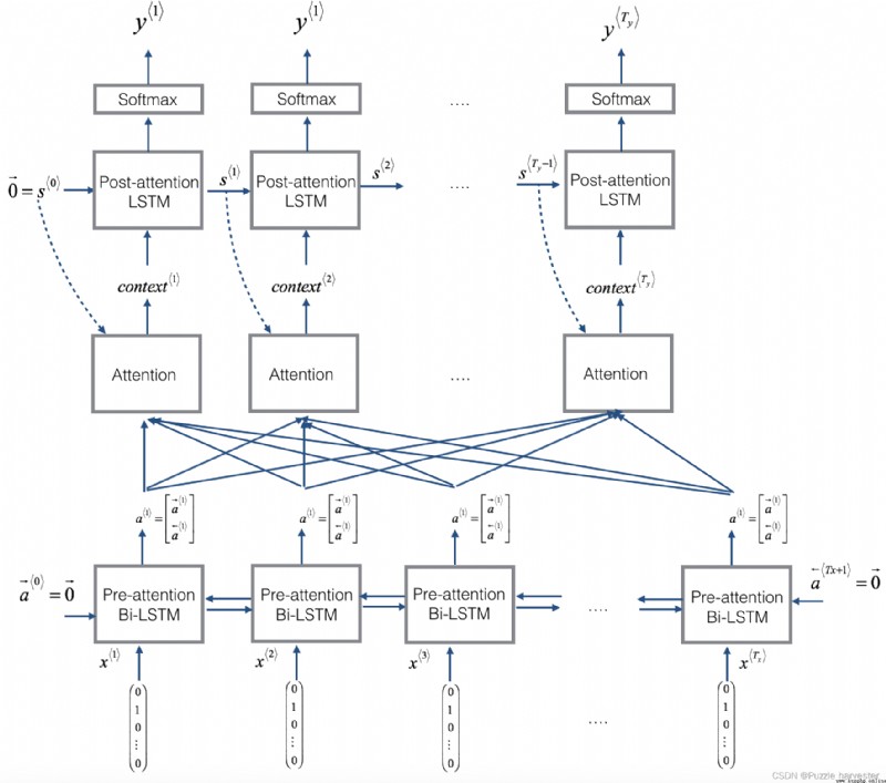
圖1:帶注意力機制的神經機器翻譯
你可能會注意到以下一些模型屬性:
RepeatVector節點復制 s * t − 1 * s^{\langle t-1 \rangle} s*t−1*的值 T x T_x Tx次,然後使用Concatenation來連接 s * t − 1 * s^{\langle t-1 \rangle} s*t−1*和 a * t * a^{\langle t \rangle} a*t*來計算 e * t , t ′ * e^{\langle t, t'\rangle} e*t,t′*,,然後將其傳遞給softmax以計算 α * t , t ′ * \alpha^{\langle t, t' \rangle} α*t,t′*。我們將在下面的Keras中說明如何使用RepeatVector和Concatenation。讓我們實現這個模型。你將從實現one_step_attention()和model()兩個函數開始:
1. one_step_attention():在步驟 t t t中,給出Bi-LSTM的所有隱藏狀態( [ a < 1 > , a < 2 > , . . . , a < T x > ] [a^{<1>},a^{<2>}, ..., a^{<T_x>}] [a<1>,a<2>,...,a<Tx>])和第二個LSTM的先前隱藏狀態( s < t − 1 > s^{<t-1>} s<t−1>),one_step_attention()將計算注意力權( [ α < t , 1 > , α < t , 2 > , . . . , α < t , T x > ] [\alpha^{<t,1>},\alpha^{<t,2>}, ..., \alpha^{<t,T_x>}] [α<t,1>,α<t,2>,...,α<t,Tx>])並輸出上下文向量(詳細信息請參見圖(右)): c o n t e x t < t > = ∑ t ′ = 0 T x α < t , t ′ > a < t ′ > (1) context^{<t>} = \sum_{t' = 0}^{T_x} \alpha^{<t,t'>}a^{<t'>}\tag{1} context<t>=t′=0∑Txα<t,t′>a<t′>(1)
請注意,我們在此筆記本中將注意力表示為 c o n t e x t * t * context^{\langle t \rangle} context*t*。在講座視頻中,上下文被表示為 c * t * c^{\langle t \rangle} c*t*,但在這裡我們將其稱為 c o n t e x t * t * context^{\langle t \rangle} context*t*,以避免與(post-attention)LSTM內部記憶單元變量混淆,有時也稱為 c * t * c^{\langle t \rangle} c*t*。
2. model():實現整個模型。它首先通過Bi-LSTM運行輸入以獲取 [ a < 1 > , a < 2 > , . . . , a < T x > ] [a^{<1>},a^{<2>}, ..., a^{<T_x>}] [a<1>,a<2>,...,a<Tx>]然後,它調用one_step_attention() T y T_y Ty次(“for”循環)。在此循環的每次迭代中,它將計算出上下文向量 c < t > c^{<t>} c<t>提供給第二個LSTM,並通過具有 s o f t m a x softmax softmax激活的密集層運行LSTM的輸出,以生成預測 y ^ < t > \hat{y}^{<t>} y^<t>。
練習:實現one_step_attention()。函數model()將使用for循環調用one_step_attention() T y T_y Ty中的層,重要的是所有 T y T_y Ty副本具有相同的權重。即,它不應該每次都重新初始化權重。換句話說,所有 T y T_y Ty步驟均應具有權重。這是在Keras中實現可共享權重的層的方法:
我們已經將你需要的層定義為全局變量。請運行以下單元格以創建它們。請檢查Keras文檔以確保你了解這些層是什麼:RepeatVector(), Concatenate(), Dense(), Activation(), Dot()。
# 將共享層定義為全局變量
repeator = RepeatVector(Tx)
concatenator = Concatenate(axis=-1)
densor1 = Dense(10, activation = "tanh")
densor2 = Dense(1, activation = "relu")
activator = Activation(softmax, name='attention_weights') # 在這個 notebook 我們正在使用自定義的 softmax(axis = 1)
dotor = Dot(axes = 1)
現在你可以使用這些層來實現one_step_attention()。 為了通過這些層之一傳播Keras張量對象X,請使用layer(X)(如果需要多個輸入則使用layer([X,Y]))。ensor(X)將通過上面定義的Dense(1)層傳播X。
# GRADED FUNCTION: one_step_attention
def one_step_attention(a, s_prev):
""" 執行一步 attention: 輸出一個上下文向量,輸出作為注意力權重的點積計算的上下文向量 "alphas" Bi-LSTM的 隱藏狀態 "a" 參數: a -- Bi-LSTM的輸出隱藏狀態 numpy-array 維度 (m, Tx, 2*n_a) s_prev -- (post-attention) LSTM的前一個隱藏狀態, numpy-array 維度(m, n_s) 返回: context -- 上下文向量, 下一個(post-attetion) LSTM 單元的輸入 """
# 使用 repeator 重復 s_prev 維度 (m, Tx, n_s) 這樣你就可以將它與所有隱藏狀態"a" 連接起來。 (≈ 1 line)
s_prev = repeator(s_prev)
# 使用 concatenator 在最後一個軸上連接 a 和 s_prev (≈ 1 line)
concat = concatenator([a, s_prev])
# 使用 densor1 傳入參數 concat, 通過一個小的全連接神經網絡來計算“中間能量”變量 e。(≈1 lines)
e = densor1(concat)
# 使用 densor2 傳入參數 e , 通過一個小的全連接神經網絡來計算“能量”變量 energies。(≈1 lines)
energies = densor2(e)
# 使用 activator 傳入參數 "energies" 計算注意力權重 "alphas" (≈ 1 line)
alphas = activator(energies)
# 使用 dotor 傳入參數 "alphas" 和 "a" 計算下一個((post-attention) LSTM 單元的上下文向量 (≈ 1 line)
context = dotor([alphas, a])
return context
在對model()函數進行編碼之後,你將能夠檢查one_step_attention()的預期輸出。
練習:按照圖2和上面的文字中的說明實現model()。再次,我們定義了全局層,這些全局層將共享將在model()中使用的權重。
n_a = 32
n_s = 64
post_activation_LSTM_cell = LSTM(n_s, return_state = True)
output_layer = Dense(len(machine_vocab), activation=softmax)
現在你可以在for循環中使用這些層 T y T_y Ty次來生成輸出,並且它們的參數將不會重新初始化。你將必須執行以下步驟:
one_step_attention()以獲取上下文向量 c o n t e x t < t > context^{<t>} context<t>。initial_state= [previous hidden state, previous cell state]傳遞此LSTM的前一個隱藏狀態 s * t − 1 * s^{\langle t-1\rangle} s*t−1*和單元狀態 c * t − 1 * c^{\langle t-1\rangle} c*t−1*。取回新的隱藏狀態 s < t > s^{<t>} s<t>和新的單元狀態 c < t > c^{<t>} c<t>。# GRADED FUNCTION: model
def model(Tx, Ty, n_a, n_s, human_vocab_size, machine_vocab_size):
""" 參數: Tx -- 輸入序列的長度 Ty -- 輸出序列的長度 n_a -- Bi-LSTM的隱藏狀態大小 n_s -- post-attention LSTM的隱藏狀態大小 human_vocab_size -- python字典 "human_vocab" 的大小 machine_vocab_size -- python字典 "machine_vocab" 的大小 返回: model -- Keras 模型實例 """
# 定義模型的輸入,維度 (Tx,)
# 定義 s0 和 c0, 初始化解碼器 LSTM 的隱藏狀態,維度 (n_s,)
X = Input(shape=(Tx, human_vocab_size))
s0 = Input(shape=(n_s,), name='s0')
c0 = Input(shape=(n_s,), name='c0')
s = s0
c = c0
# 初始化一個空的輸出列表
outputs = []
# 第一步:定義 pre-attention Bi-LSTM。 記得使用 return_sequences=True. (≈ 1 line)
a = Bidirectional(LSTM(n_a, return_sequences=True), input_shape=(m, Tx, n_a * 2))(X)
# 第二步:迭代 Ty 步
for t in range(Ty):
# 第二步.A: 執行一步注意機制,得到在 t 步的上下文向量 (≈ 1 line)
context = one_step_attention(a, s)
# 第二步.B: 使用 post-attention LSTM 單元得到新的 "context"
# 別忘了使用: initial_state = [hidden state, cell state] (≈ 1 line)
s, _, c = post_activation_LSTM_cell(context, initial_state=[s, c])
# 第二步.C: 使用全連接層處理post-attention LSTM 的隱藏狀態輸出 (≈ 1 line)
out = output_layer(s)
# 第二步.D: 追加 "out" 到 "outputs" 列表 (≈ 1 line)
outputs.append(out)
# 第三步:創建模型實例,獲取三個輸入並返回輸出列表。 (≈ 1 line)
model = Model(inputs=[X, s0, c0], outputs=outputs)
return model
運行以下單元以創建模型。
model = model(Tx, Ty, n_a, n_s, len(human_vocab), len(machine_vocab))
WARNING:tensorflow:From d:\vr\virtual_environment\lib\site-packages\tensorflow_core\python\ops\resource_variable_ops.py:1630: calling BaseResourceVariable.__init__ (from tensorflow.python.ops.resource_variable_ops) with constraint is deprecated and will be removed in a future version.
Instructions for updating:
If using Keras pass *_constraint arguments to layers.
讓我們獲得模型的總結,以檢查其是否與預期輸出匹配。
model.summary()
Model: "model_1"
__________________________________________________________________________________________________
Layer (type) Output Shape Param # Connected to
==================================================================================================
input_1 (InputLayer) (None, 30, 37) 0
__________________________________________________________________________________________________
s0 (InputLayer) (None, 64) 0
__________________________________________________________________________________________________
bidirectional_1 (Bidirectional) (None, 30, 64) 17920 input_1[0][0]
__________________________________________________________________________________________________
repeat_vector_1 (RepeatVector) (None, 30, 64) 0 s0[0][0]
lstm_1[0][0]
lstm_1[1][0]
lstm_1[2][0]
lstm_1[3][0]
lstm_1[4][0]
lstm_1[5][0]
lstm_1[6][0]
lstm_1[7][0]
lstm_1[8][0]
__________________________________________________________________________________________________
concatenate_1 (Concatenate) (None, 30, 128) 0 bidirectional_1[0][0]
repeat_vector_1[0][0]
bidirectional_1[0][0]
repeat_vector_1[1][0]
bidirectional_1[0][0]
repeat_vector_1[2][0]
bidirectional_1[0][0]
repeat_vector_1[3][0]
bidirectional_1[0][0]
repeat_vector_1[4][0]
bidirectional_1[0][0]
repeat_vector_1[5][0]
bidirectional_1[0][0]
repeat_vector_1[6][0]
bidirectional_1[0][0]
repeat_vector_1[7][0]
bidirectional_1[0][0]
repeat_vector_1[8][0]
bidirectional_1[0][0]
repeat_vector_1[9][0]
__________________________________________________________________________________________________
dense_1 (Dense) (None, 30, 10) 1290 concatenate_1[0][0]
concatenate_1[1][0]
concatenate_1[2][0]
concatenate_1[3][0]
concatenate_1[4][0]
concatenate_1[5][0]
concatenate_1[6][0]
concatenate_1[7][0]
concatenate_1[8][0]
concatenate_1[9][0]
__________________________________________________________________________________________________
dense_2 (Dense) (None, 30, 1) 11 dense_1[0][0]
dense_1[1][0]
dense_1[2][0]
dense_1[3][0]
dense_1[4][0]
dense_1[5][0]
dense_1[6][0]
dense_1[7][0]
dense_1[8][0]
dense_1[9][0]
__________________________________________________________________________________________________
attention_weights (Activation) (None, 30, 1) 0 dense_2[0][0]
dense_2[1][0]
dense_2[2][0]
dense_2[3][0]
dense_2[4][0]
dense_2[5][0]
dense_2[6][0]
dense_2[7][0]
dense_2[8][0]
dense_2[9][0]
__________________________________________________________________________________________________
dot_1 (Dot) (None, 1, 64) 0 attention_weights[0][0]
bidirectional_1[0][0]
attention_weights[1][0]
bidirectional_1[0][0]
attention_weights[2][0]
bidirectional_1[0][0]
attention_weights[3][0]
bidirectional_1[0][0]
attention_weights[4][0]
bidirectional_1[0][0]
attention_weights[5][0]
bidirectional_1[0][0]
attention_weights[6][0]
bidirectional_1[0][0]
attention_weights[7][0]
bidirectional_1[0][0]
attention_weights[8][0]
bidirectional_1[0][0]
attention_weights[9][0]
bidirectional_1[0][0]
__________________________________________________________________________________________________
c0 (InputLayer) (None, 64) 0
__________________________________________________________________________________________________
lstm_1 (LSTM) [(None, 64), (None, 33024 dot_1[0][0]
s0[0][0]
c0[0][0]
dot_1[1][0]
lstm_1[0][0]
lstm_1[0][2]
dot_1[2][0]
lstm_1[1][0]
lstm_1[1][2]
dot_1[3][0]
lstm_1[2][0]
lstm_1[2][2]
dot_1[4][0]
lstm_1[3][0]
lstm_1[3][2]
dot_1[5][0]
lstm_1[4][0]
lstm_1[4][2]
dot_1[6][0]
lstm_1[5][0]
lstm_1[5][2]
dot_1[7][0]
lstm_1[6][0]
lstm_1[6][2]
dot_1[8][0]
lstm_1[7][0]
lstm_1[7][2]
dot_1[9][0]
lstm_1[8][0]
lstm_1[8][2]
__________________________________________________________________________________________________
dense_3 (Dense) (None, 11) 715 lstm_1[0][0]
lstm_1[1][0]
lstm_1[2][0]
lstm_1[3][0]
lstm_1[4][0]
lstm_1[5][0]
lstm_1[6][0]
lstm_1[7][0]
lstm_1[8][0]
lstm_1[9][0]
==================================================================================================
Total params: 52,960
Trainable params: 52,960
Non-trainable params: 0
__________________________________________________________________________________________________
與往常一樣,在Keras中創建模型後,你需要對其進行編譯並定義要使用的損失,優化器和評價指標。 使用categorical_crossentropy損失,自定義Adam、optimizer(learning rate = 0.005, β 1 = 0.9 \beta_1 = 0.9 β1=0.9, β 2 = 0.999 \beta_2 = 0.999 β2=0.999, decay = 0.01)和['accuracy']指標:
### START CODE HERE ### (≈2 lines)
opt = Adam(lr=0.005, beta_1=0.9, beta_2=0.999, decay=0.01)
model.compile(loss='categorical_crossentropy', optimizer=opt, metrics=['accuracy'])
### END CODE HERE ###
最後一步是定義所有輸入和輸出以適合模型:
s0和c0以將你的post_activation_LSTM_cell初始化為0。model(),你需要"outputs"作為11個維度元素 ( m , T y ) (m,T_y) (m,Ty)的列表。因此:outputs[i][0], ..., outputs[i][Ty]代表與訓練示例(X[i])。更一般而言, outputs[i][j]是 i t h i^{th} ith訓練示例中 j t h j^{th} jth字符的真實標簽。s0 = np.zeros((m, n_s))
c0 = np.zeros((m, n_s))
outputs = list(Yoh.swapaxes(0,1))
現在讓我們擬合模型並運行一個epoch。
model.fit([Xoh, s0, c0], outputs, epochs=1, batch_size=100)
WARNING:tensorflow:From d:\vr\virtual_environment\lib\site-packages\keras\backend\tensorflow_backend.py:422: The name tf.global_variables is deprecated. Please use tf.compat.v1.global_variables instead.
Epoch 1/1
10000/10000 [==============================] - 10s 974us/step - loss: 16.9091 - dense_3_loss: 2.6079 - dense_3_accuracy: 0.5427 - dense_3_accuracy_1: 0.6577 - dense_3_accuracy_2: 0.2775 - dense_3_accuracy_3: 0.0766 - dense_3_accuracy_4: 0.9821 - dense_3_accuracy_5: 0.3126 - dense_3_accuracy_6: 0.0482 - dense_3_accuracy_7: 0.9545 - dense_3_accuracy_8: 0.2243 - dense_3_accuracy_9: 0.0955
<keras.callbacks.callbacks.History at 0x272a6daafd0>
訓練時,你可以看到輸出的10個位置中的每個位置的損失以及准確性。下表為你提供了一個示例,說明該批次有2個示例時的精確度:
因此,dense_2_acc_8: 0.89意味著你在當前數據批次中有89%的時間正確預測了輸出的第7個字符。
我們對該模型運行了更長的時間,並節省了權重。運行下一個單元格以加載我們的體重。(通過訓練模型幾分鐘,你應該可以獲得准確度相似的模型,但是加載我們的模型可以節省你的時間。)
model.load_weights('models/model.h5')
現在,你可以在新示例中查看結果。
EXAMPLES = ['3 May 1979', '5 April 09', '21th of August 2016', 'Tue 10 Jul 2007', 'Saturday May 9 2018', 'March 3 2001', 'March 3rd 2001', '1 March 2001']
for example in EXAMPLES:
source = string_to_int(example, Tx, human_vocab)
source = np.array(list(map(lambda x: to_categorical(x, num_classes=len(human_vocab)), source)))
prediction = model.predict([[source], s0, c0])
prediction = np.argmax(prediction, axis = -1)
output = [inv_machine_vocab[int(i)] for i in prediction]
print("source:", example)
print("output:", ''.join(output))
source: 3 May 1979
output: 1979-05-33
source: 5 April 09
output: 2009-04-05
source: 21th of August 2016
output: 2016-08-20
source: Tue 10 Jul 2007
output: 2007-07-10
source: Saturday May 9 2018
output: 2018-05-09
source: March 3 2001
output: 2001-03-03
source: March 3rd 2001
output: 2001-03-03
source: 1 March 2001
output: 2001-03-01
你也可以更改這些示例,以使用自己的示例進行測試。下一部分將使你更好地了解注意力機制的作用-即生成特定輸出字符時網絡要注意的輸入部分。
由於問題的輸出長度固定為10,因此還可以使用10個不同的softmax單元來執行此任務,以生成10個字符的輸出。但是注意力模型的一個優點是輸出的每個部分(例如月份)都知道它只需要依賴輸入的一小部分(輸入中代表月份的字符)。我們可以可視化輸出的哪一部分正在查看輸入的哪一部分。
考慮將"Saturday 9 May 2018"轉換為"2018-05-09"的任務。如果我們可視化計算出的 α * t , t ′ * \alpha^{\langle t, t' \rangle} α*t,t′*,我們將得到:
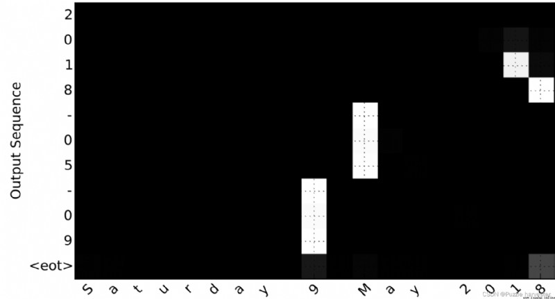
圖8: 完整的注意圖
注意輸出如何忽略輸入的"Saturday"部分。沒有一個輸出時間步長關注輸入的那部分。我們還看到9已被翻譯為09,May已被正確翻譯為05,而輸出則注意進行翻譯所需的部分輸入。該年份主要要求它注意輸入的“18”以生成“2018”。
現在讓我們可視化你網絡中的注意力值。我們將通過網絡傳播一個示例,然後可視化 α * t , t ′ * \alpha^{\langle t, t' \rangle} α*t,t′*的值。
為了弄清注意值的位置,讓我們開始打印模型摘要。
model.summary()
Model: "model_1"
__________________________________________________________________________________________________
Layer (type) Output Shape Param # Connected to
==================================================================================================
input_1 (InputLayer) (None, 30, 37) 0
__________________________________________________________________________________________________
s0 (InputLayer) (None, 64) 0
__________________________________________________________________________________________________
bidirectional_1 (Bidirectional) (None, 30, 64) 17920 input_1[0][0]
__________________________________________________________________________________________________
repeat_vector_1 (RepeatVector) (None, 30, 64) 0 s0[0][0]
lstm_1[0][0]
lstm_1[1][0]
lstm_1[2][0]
lstm_1[3][0]
lstm_1[4][0]
lstm_1[5][0]
lstm_1[6][0]
lstm_1[7][0]
lstm_1[8][0]
__________________________________________________________________________________________________
concatenate_1 (Concatenate) (None, 30, 128) 0 bidirectional_1[0][0]
repeat_vector_1[0][0]
bidirectional_1[0][0]
repeat_vector_1[1][0]
bidirectional_1[0][0]
repeat_vector_1[2][0]
bidirectional_1[0][0]
repeat_vector_1[3][0]
bidirectional_1[0][0]
repeat_vector_1[4][0]
bidirectional_1[0][0]
repeat_vector_1[5][0]
bidirectional_1[0][0]
repeat_vector_1[6][0]
bidirectional_1[0][0]
repeat_vector_1[7][0]
bidirectional_1[0][0]
repeat_vector_1[8][0]
bidirectional_1[0][0]
repeat_vector_1[9][0]
__________________________________________________________________________________________________
dense_1 (Dense) (None, 30, 10) 1290 concatenate_1[0][0]
concatenate_1[1][0]
concatenate_1[2][0]
concatenate_1[3][0]
concatenate_1[4][0]
concatenate_1[5][0]
concatenate_1[6][0]
concatenate_1[7][0]
concatenate_1[8][0]
concatenate_1[9][0]
__________________________________________________________________________________________________
dense_2 (Dense) (None, 30, 1) 11 dense_1[0][0]
dense_1[1][0]
dense_1[2][0]
dense_1[3][0]
dense_1[4][0]
dense_1[5][0]
dense_1[6][0]
dense_1[7][0]
dense_1[8][0]
dense_1[9][0]
__________________________________________________________________________________________________
attention_weights (Activation) (None, 30, 1) 0 dense_2[0][0]
dense_2[1][0]
dense_2[2][0]
dense_2[3][0]
dense_2[4][0]
dense_2[5][0]
dense_2[6][0]
dense_2[7][0]
dense_2[8][0]
dense_2[9][0]
__________________________________________________________________________________________________
dot_1 (Dot) (None, 1, 64) 0 attention_weights[0][0]
bidirectional_1[0][0]
attention_weights[1][0]
bidirectional_1[0][0]
attention_weights[2][0]
bidirectional_1[0][0]
attention_weights[3][0]
bidirectional_1[0][0]
attention_weights[4][0]
bidirectional_1[0][0]
attention_weights[5][0]
bidirectional_1[0][0]
attention_weights[6][0]
bidirectional_1[0][0]
attention_weights[7][0]
bidirectional_1[0][0]
attention_weights[8][0]
bidirectional_1[0][0]
attention_weights[9][0]
bidirectional_1[0][0]
__________________________________________________________________________________________________
c0 (InputLayer) (None, 64) 0
__________________________________________________________________________________________________
lstm_1 (LSTM) [(None, 64), (None, 33024 dot_1[0][0]
s0[0][0]
c0[0][0]
dot_1[1][0]
lstm_1[0][0]
lstm_1[0][2]
dot_1[2][0]
lstm_1[1][0]
lstm_1[1][2]
dot_1[3][0]
lstm_1[2][0]
lstm_1[2][2]
dot_1[4][0]
lstm_1[3][0]
lstm_1[3][2]
dot_1[5][0]
lstm_1[4][0]
lstm_1[4][2]
dot_1[6][0]
lstm_1[5][0]
lstm_1[5][2]
dot_1[7][0]
lstm_1[6][0]
lstm_1[6][2]
dot_1[8][0]
lstm_1[7][0]
lstm_1[7][2]
dot_1[9][0]
lstm_1[8][0]
lstm_1[8][2]
__________________________________________________________________________________________________
dense_3 (Dense) (None, 11) 715 lstm_1[0][0]
lstm_1[1][0]
lstm_1[2][0]
lstm_1[3][0]
lstm_1[4][0]
lstm_1[5][0]
lstm_1[6][0]
lstm_1[7][0]
lstm_1[8][0]
lstm_1[9][0]
==================================================================================================
Total params: 52,960
Trainable params: 52,960
Non-trainable params: 0
__________________________________________________________________________________________________
浏覽上面的model.summary()的輸出。你可以看到,在每個時間步dot_2計算 t = 0 , … , T y − 1 t = 0, \ldots, T_y-1 t=0,…,Ty−1上下文向量之前,名為attention_weights的層都會輸出維度為 ( m , 30 , 1 ) (m, 30, 1) (m,30,1)的alphas。讓我們從該層獲取激活。
函數attention_map()從模型中提取注意力值並繪制它們。
attention_map = plot_attention_map(model, human_vocab, inv_machine_vocab, "Tuesday 09 Oct 1993", num = 7, n_s = 64)
<Figure size 432x288 with 0 Axes>
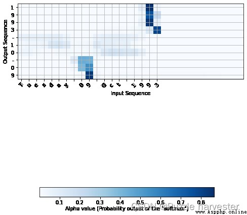
在生成的圖上,你可以觀察預測輸出的每個字符的注意權重值。檢查此圖,並檢查網絡對你的關注是否有意義。
在日期轉換應用程序中,你會發現大部分時間的注意力都有助於預測年份,並且對預測日期/月份沒有太大影響。
這是你在此筆記本中應記住的內容: