此次你將使用單詞向量表示來構建Emojifier表情符號。
你是否曾經想過讓短信更具表現力?你的emojifier應用程序將幫助你做到這一點。因此,與其寫“恭喜晉升!有機會喝杯咖啡聊天吧。愛你!” emojifier可以自動將其變成“恭喜升職!有機會一起喝咖啡️聊天吧,愛你!️”
你將實現一個模型,該模型輸入一個句子(例如“讓我們今晚去看棒球比賽!”),並找到最適合與該句子搭配使用的表情符號(️)。在許多表情符號界面中,你需要記住️是“心”符號而不是“愛”符號。但是使用單詞向量,你會看到,即使你的訓練集僅將幾個單詞與特定表情符號明確關聯,你的算法也能夠將測試集中的單詞歸納並關聯到同一表情符號,即使這些單詞沒有甚至不會出現在訓練集中。這樣,即使使用很小的訓練集,也可以構建從句子到表情符號的准確分類器映射。
在本練習中,你將從使用單詞嵌入的基准模型(Emojifier-V1)開始,然後構建一個包含LSTM的更復雜的模型(Emojifier-V2)。
import numpy as np
from emo_utils import *
import emoji
import matplotlib.pyplot as plt
%matplotlib inline
讓我們從構建一個簡單的baseline分類器開始。
你有一個很小的數據集(X,Y),其中:
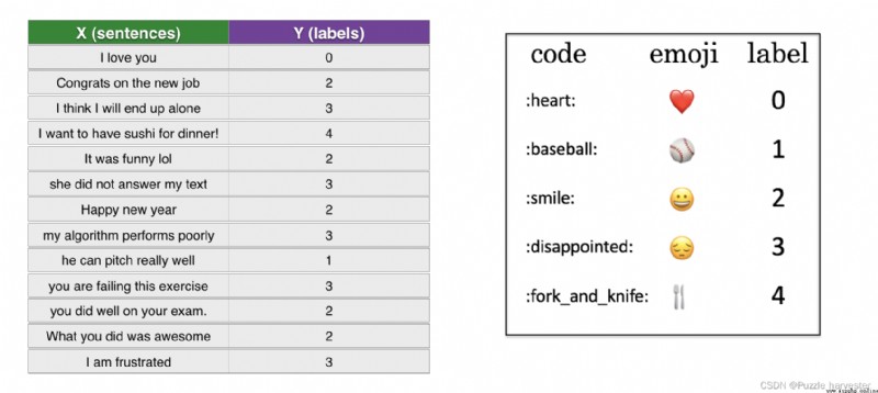
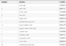
圖1 :EemoSet-5分類問題。這裡列出了一些例句。
讓我們使用下面的代碼加載數據集。我們將數據集分為訓練(127個示例)和測試(56個示例)集。
X_train, Y_train = read_csv('data/train_emoji.csv')
X_test, Y_test = read_csv('data/tesss.csv')
aa = max(X_train, key=len);
maxLen = len(max(X_train, key=len).split())
運行以下單元格以打印X_train和Y_train的句子的相應標簽。更改index以查看不同的示例。由於iPython筆記本使用的字體,愛心表情符號可能會是黑色而不是紅色。
如果下面出現問題,檢查一下emoji的版本是不是0.5.4
index = 5
print(X_train[index], label_to_emoji(Y_train[index]))
I love you mum ️
在這一部分中,你將實現一個稱為“Emojifier-v1”的基准模型。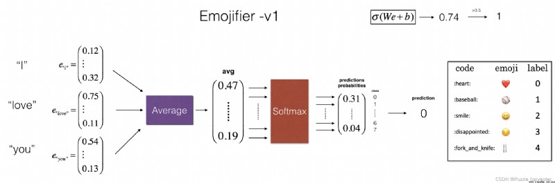
圖2 :基准模型(Emojifier-V1)。
模型的輸入是與句子相對應的字符串(例如,“I love you”。在代碼中,輸出將是維度為(1,5)的概率向量,然後將其傳遞到argmax層中以提取概率最大的表情符號的輸出索引。
為了使我們的標簽成為適合訓練softmax分類器的格式,讓我們將從當前 Y Y Y的維度、 ( m , 1 ) (m,1) (m,1)轉換為"one-hot表示" ( m , 5 ) (m,5) (m,5),其中每個row是一個one-hot向量,提供了一個示例的標簽,你可以使用下一個代碼截取器來實現。在這裡,Y_oh在變量名Y_oh_train和Y_oh_test中代表"Y-one-hot" :
Y_oh_train = convert_to_one_hot(Y_train, C = 5)
Y_oh_test = convert_to_one_hot(Y_test, C = 5)
讓我們看看convert_to_one_hot()做了什麼。隨時更改index以輸出不同的值。
index = 50
print(Y_train[index], "is converted into one hot", Y_oh_train[index])
0 is converted into one hot [1. 0. 0. 0. 0.]
現在,所有數據都准備好輸入到Emojify-V1模型。讓我們實現模型!
如圖(2)所示,第一步是將輸入句子轉換為單詞向量表示形式,然後將它們平均在一起。與之前的練習類似,我們將使用預訓練的50維GloVe嵌入。運行以下單元格以加載word_to_vec_map,其中包含所有向量表示形式。
word_to_index, index_to_word, word_to_vec_map = read_glove_vecs('data/glove.6B.50d.txt')
你已加載:
word_to_index:字典將單詞映射到詞匯表中的索引(400,001個單詞,有效索引范圍是0到400,000)index_to_word:字典從索引到詞匯表中對應詞的映射word_to_vec_map:將單詞映射到其GloVe向量表示的字典。運行以下單元格以檢查其是否有效。
word = "cucumber"
index = 289846
print("the index of", word, "in the vocabulary is", word_to_index[word])
print("the", str(index) + "th word in the vocabulary is", index_to_word[index])
the index of cucumber in the vocabulary is 113315
the 289846th word in the vocabulary is potboiler
練習:實現sentence_to_avg(),你將需要執行兩個步驟:
X.lower()和X.split()可能有用。def sentence_to_avg(sentence, word_to_vec_map):
""" 將句子轉換為單詞列表,提取其GloVe向量,然後將其平均。 參數: sentence -- 字符串類型,從X中獲取的樣本。 word_to_vec_map -- 字典類型,單詞映射到50維的向量的字典 返回: avg -- 對句子的均值編碼,維度為(50,) """
# 第一步:分割句子,轉換為列表。
words = sentence.lower().split()
# 初始化均值詞向量
avg = np.zeros(50,)
# 第二步:對詞向量取平均。
for w in words:
avg += word_to_vec_map[w]
avg = np.divide(avg, len(words))
return avg
avg = sentence_to_avg("Morrocan couscous is my favorite dish", word_to_vec_map)
print("avg = ", avg)
avg = [-0.008005 0.56370833 -0.50427333 0.258865 0.55131103 0.03104983
-0.21013718 0.16893933 -0.09590267 0.141784 -0.15708967 0.18525867
0.6495785 0.38371117 0.21102167 0.11301667 0.02613967 0.26037767
0.05820667 -0.01578167 -0.12078833 -0.02471267 0.4128455 0.5152061
0.38756167 -0.898661 -0.535145 0.33501167 0.68806933 -0.2156265
1.797155 0.10476933 -0.36775333 0.750785 0.10282583 0.348925
-0.27262833 0.66768 -0.10706167 -0.283635 0.59580117 0.28747333
-0.3366635 0.23393817 0.34349183 0.178405 0.1166155 -0.076433
0.1445417 0.09808667]
模型
現在,你已經完成了所有實現model()函數的步驟。使用sentence_to_avg()之後,你需要使平均值通過正向傳播,計算損失,然後反向傳播以更新softmax的參數。
練習:實現圖(2)中描述的model()函數。假設 Y o h Y_{oh} Yoh(“Y獨熱”)是輸出標簽的獨熱編碼,則在正向傳遞中需要實現的公式和計算交叉熵損失的公式為:
z ( i ) = W . a v g ( i ) + b z^{(i)} = W . avg^{(i)} + b z(i)=W.avg(i)+b
a ( i ) = s o f t m a x ( z ( i ) ) a^{(i)} = softmax(z^{(i)}) a(i)=softmax(z(i))
L ( i ) = − ∑ k = 0 n y − 1 Y o h , k ( i ) ∗ l o g ( a k ( i ) ) \mathcal{L}^{(i)} = - \sum_{k = 0}^{n_y - 1} Y_{oh,k}^{(i)} * log(a^{(i)}_k) L(i)=−k=0∑ny−1Yoh,k(i)∗log(ak(i))
有可能提出一個更有效的向量化實現。但是,由於我們始終使用for循環將句子一次轉換為 a v g ( i ) avg^{(i)} avg(i)表示形式,因此這次我們不用理會。
我們為你提供了一個函數softmax()。
def model(X, Y, word_to_vec_map, learning_rate=0.01, num_iterations=400):
""" 在numpy中訓練詞向量模型。 參數: X -- 輸入的字符串類型的數據,維度為(m, 1)。 Y -- 對應的標簽,0-7的數組,維度為(m, 1)。 word_to_vec_map -- 字典類型的單詞到50維詞向量的映射。 learning_rate -- 學習率. num_iterations -- 迭代次數。 返回: pred -- 預測的向量,維度為(m, 1)。 W -- 權重參數,維度為(n_y, n_h)。 b -- 偏置參數,維度為(n_y,) """
np.random.seed(1)
# 定義訓練數量
m = Y.shape[0]
n_y = 5
n_h = 50
# 使用Xavier初始化參數
W = np.random.randn(n_y, n_h) / np.sqrt(n_h)
b = np.zeros((n_y,))
# 將Y轉換成獨熱編碼
Y_oh = convert_to_one_hot(Y, C=n_y)
# 優化循環
for t in range(num_iterations):
for i in range(m):
# 獲取第i個訓練樣本的均值
avg = sentence_to_avg(X[i], word_to_vec_map)
# 前向傳播
z = np.dot(W, avg) + b
a = softmax(z)
# 計算第i個訓練的損失
cost = -np.sum(Y_oh[i]*np.log(a))
# 計算梯度
dz = a - Y_oh[i]
dW = np.dot(dz.reshape(n_y,1), avg.reshape(1, n_h))
db = dz
# 更新參數
W = W - learning_rate * dW
b = b - learning_rate * db
if t % 100 == 0:
print("第{t}輪,損失為{cost}".format(t=t,cost=cost))
pred = predict(X, Y, W, b, word_to_vec_map)
return pred, W, b
print(X_train.shape)
print(Y_train.shape)
print(np.eye(5)[Y_train.reshape(-1)].shape)
print(X_train[0])
print(type(X_train))
Y = np.asarray([5,0,0,5, 4, 4, 4, 6, 6, 4, 1, 1, 5, 6, 6, 3, 6, 3, 4, 4])
print(Y.shape)
X = np.asarray(['I am going to the bar tonight', 'I love you', 'miss you my dear',
'Lets go party and drinks','Congrats on the new job','Congratulations',
'I am so happy for you', 'Why are you feeling bad', 'What is wrong with you',
'You totally deserve this prize', 'Let us go play football',
'Are you down for football this afternoon', 'Work hard play harder',
'It is suprising how people can be dumb sometimes',
'I am very disappointed','It is the best day in my life',
'I think I will end up alone','My life is so boring','Good job',
'Great so awesome'])
(132,)
(132,)
(132, 5)
never talk to me again
<class 'numpy.ndarray'>
(20,)
運行下一個單元格來訓練模型並學習softmax參數(W,b)。
pred, W, b = model(X_train, Y_train, word_to_vec_map)
print(pred.T)
第0輪,損失為1.9520498812810072
Accuracy: 0.3484848484848485
第100輪,損失為0.07971818726014807
Accuracy: 0.9318181818181818
第200輪,損失為0.04456369243681402
Accuracy: 0.9545454545454546
第300輪,損失為0.03432267378786059
Accuracy: 0.9696969696969697
[[3. 2. 3. 0. 4. 0. 3. 2. 3. 1. 3. 3. 1. 3. 2. 3. 2. 3. 1. 2. 3. 0. 2. 2.
2. 1. 4. 3. 3. 4. 0. 3. 4. 2. 0. 3. 2. 2. 3. 4. 2. 2. 0. 2. 3. 0. 3. 2.
4. 3. 0. 3. 3. 3. 4. 2. 1. 1. 1. 2. 3. 1. 0. 0. 0. 3. 4. 4. 2. 2. 1. 2.
0. 3. 2. 2. 0. 3. 3. 1. 2. 1. 2. 2. 4. 3. 3. 2. 4. 0. 0. 3. 3. 3. 3. 2.
0. 1. 2. 3. 0. 2. 2. 2. 3. 2. 2. 2. 4. 1. 1. 3. 3. 4. 1. 2. 1. 1. 3. 1.
0. 4. 0. 3. 3. 4. 4. 1. 4. 3. 0. 2.]]
Great!你的模型在訓練集上具有很高的准確性。現在讓我們看看它如何在測試集上運行。
print("=====訓練集====")
pred_train = predict(X_train, Y_train, W, b, word_to_vec_map)
print("=====測試集====")
pred_test = predict(X_test, Y_test, W, b, word_to_vec_map)
=====訓練集====
Accuracy: 0.9772727272727273
=====測試集====
Accuracy: 0.8571428571428571
假設有5個類別,那麼隨機猜測的准確率將達到20%。在僅訓練了127個示例之後,這是相當不錯的表現。
在訓練集中,算法看到帶有標簽️的句子"I love you"。但是,你可以檢查單詞"adore"是否沒有出現在訓練集中。盡管如此,讓我們看看如果你寫"I adore you."會發生什麼。
X_my_sentences = np.array(["i adore you", "i love you", "funny lol", "lets play with a ball", "food is ready", "not feeling happy"])
Y_my_labels = np.array([[0], [0], [2], [1], [4],[3]])
pred = predict(X_my_sentences, Y_my_labels , W, b, word_to_vec_map)
print_predictions(X_my_sentences, pred)
Accuracy: 0.8333333333333334
i adore you ️
i love you ️
funny lol
lets play with a ball
food is ready
not feeling happy
驚人!由於adore具有與love類似的嵌入方式,因此該算法可以正確地推廣到甚至從未見過的單詞。heart,dear,beloved或adore之類的單詞具有類似於love的嵌入向量,因此也可以使用-隨意修改上面的輸入並嘗試各種輸入語句。看看效果如何?
請注意,盡管這樣並不能使"not feeling happy"正確。該算法忽略單詞順序,因此不善於理解"not happy."之類的短語。
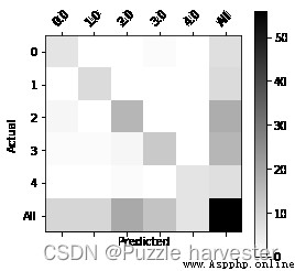
我們把矩陣打印出來應該會幫助你理解哪些類讓模型學習起來比較困難,橫軸為預測,豎軸為實際標簽。
print(Y_test.shape)
print(' '+ label_to_emoji(0)+ ' ' + label_to_emoji(1) + ' ' + label_to_emoji(2)+ ' ' + label_to_emoji(3)+' ' + label_to_emoji(4))
print(pd.crosstab(Y_test, pred_test.reshape(56,), rownames=['Actual'], colnames=['Predicted'], margins=True))
plot_confusion_matrix(Y_test, pred_test)
(56,)
️
Predicted 0.0 1.0 2.0 3.0 4.0 All
Actual
0 6 0 0 1 0 7
1 0 8 0 0 0 8
2 2 0 16 0 0 18
3 1 1 2 12 0 16
4 0 0 1 0 6 7
All 9 9 19 13 6 56
這部分你應該記住:
讓我們建立一個LSTM模型作為輸入單詞序列。此模型將能夠考慮單詞順序。Emojifier-V2將繼續使用預訓練的單詞嵌入來表示單詞,但會將其輸入到LSTM中,LSTM的工作是預測最合適的表情符號。
import numpy as np
np.random.seed(0)
from keras.models import Model
from keras.layers import Dense, Input, Dropout, LSTM, Activation
from keras.layers.embeddings import Embedding
from keras.preprocessing import sequence
from keras.initializers import glorot_uniform
np.random.seed(1)
Using TensorFlow backend.
這是你將實現的Emojifier-v2: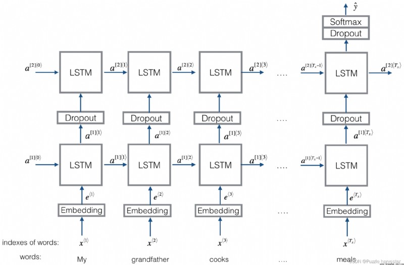
圖3 :Emojifier-V2;2層LSTM序列分類器。
在本練習中,我們想使用mini-batch訓練Keras。但是,大多數深度學習框架要求同一小批次中的所有序列具有相同的長度。這就是向量化可以起作用的原因:如果你有3個單詞的句子和4個單詞的句子,那麼它們所需的計算是不同的(一個LSTM需要3個步驟,一個LSTM需要4個步驟),所以同時做他們兩個是不可能的。
常見的解決方案是使用填充。具體來說,設置最大序列長度,並將所有序列填充為相同的長度。例如,最大序列長度為20,我們可以用“0”填充每個句子,以便每個輸入句子的長度為20。因此,句子"i love you"將表示為 ( e I , e l o v e , e y o u , 0 ⃗ , 0 ⃗ , … , 0 ⃗ ) (e_{I}, e_{love}, e_{you}, \vec{0}, \vec{0}, \ldots, \vec{0}) (eI,elove,eyou,0,0,…,0)。在此示例中,任何長度超過20個單詞的句子都必須被截斷。選擇最大序列長度的一種簡單方法是僅選擇訓練集中最長句子的長度。
在Keras中,嵌入矩陣表示為“層”,並將正整數(對應於單詞的索引)映射為固定大小的密集向量(嵌入向量)。可以使用預訓練的嵌入對其進行訓練或初始化。在這一部分中,你將學習如何在Keras中創建Embedding()層,並使用之前在筆記本中加載的GloVe 50維向量對其進行初始化。因為我們的訓練集很小,所以我們不會更新單詞嵌入,而是將其值保持不變。但是在下面的代碼中,我們將向你展示Keras如何允許你訓練或固定該層。
Embedding()層采用大小(batch size,max input length)的整數矩陣作為輸入。如下圖所示,這對應於轉換為索引列表(句子)的句子。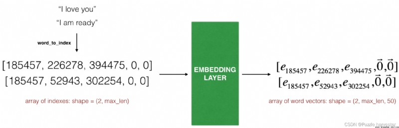
圖4:嵌入層;此示例顯示了兩個示例通過嵌入層的傳播。兩者都被零填充到max_len=5的長度。最終的向量維度為(2,max_len,50),因為我們使用的詞嵌入為50維。
輸入中的最大整數(即單詞索引)應不大於詞匯表的大小。該層輸出一個維度數組(batch size, max input length, dimension of word vectors)。
第一步是將所有訓練語句轉換為索引列表,然後對所有這些列表進行零填充,以使它們的長度為最長句子的長度。
練習:實現以下函數,將X(字符串形式的句子數組)轉換為與句子中單詞相對應的索引數組。輸出維度應使其可以賦予Embedding()(如圖4所示)。
def sentences_to_indices(X, word_to_index, max_len):
""" 輸入的是X(字符串類型的句子的數組),再轉化為對應的句子列表, 輸出的是能夠讓Embedding()函數接受的列表或矩陣(參見圖4)。 參數: X -- 句子數組,維度為(m, 1) word_to_index -- 字典類型的單詞到索引的映射 max_len -- 最大句子的長度,數據集中所有的句子的長度都不會超過它。 返回: X_indices -- 對應於X中的單詞索引數組,維度為(m, max_len) """
m = X.shape[0] # 訓練集數量
# 使用0初始化X_indices
X_indices = np.zeros((m, max_len))
for i in range(m):
# 將第i個句子轉化為小寫並按單詞分開。
sentences_words = X[i].lower().split()
# 初始化j為0
j = 0
# 遍歷這個單詞列表
for w in sentences_words:
# 將X_indices的第(i, j)號元素為對應的單詞索引
X_indices[i, j] = word_to_index[w]
j += 1
return X_indices
運行以下單元格以檢查sentences_to_indices()的作用,並檢查結果。
X1 = np.array(["funny lol", "lets play baseball", "food is ready for you"])
X1_indices = sentences_to_indices(X1,word_to_index, max_len = 5)
print("X1 =", X1)
print("X1_indices =", X1_indices)
X1 = ['funny lol' 'lets play baseball' 'food is ready for you']
X1_indices = [[155343. 225120. 0. 0. 0.]
[220928. 286370. 69714. 0. 0.]
[151202. 192971. 302249. 151347. 394463.]]
讓我們使用預先訓練的單詞向量在Keras中構建Embedding()層。建立此層後,你將把sentences_to_indices()的輸出作為輸入傳遞給它,而Embedding()層將返回句子的單詞嵌入。
練習:實現pretrained_embedding_layer()。你將需要執行以下步驟:
def pretrained_embedding_layer(word_to_vec_map, word_to_index):
""" 創建Keras Embedding()層,加載已經訓練好了的50維GloVe向量 參數: word_to_vec_map -- 字典類型的單詞與詞嵌入的映射 word_to_index -- 字典類型的單詞到詞匯表(400,001個單詞)的索引的映射。 返回: embedding_layer() -- 訓練好了的Keras的實體層。 """
vocab_len = len(word_to_index) + 1
emb_dim = word_to_vec_map["cucumber"].shape[0]
# 初始化嵌入矩陣
emb_matrix = np.zeros((vocab_len, emb_dim))
# 將嵌入矩陣的每行的“index”設置為詞匯“index”的詞向量表示
for word, index in word_to_index.items():
emb_matrix[index, :] = word_to_vec_map[word]
# 定義Keras的embbeding層
embedding_layer = Embedding(vocab_len, emb_dim, trainable=False)
# 構建embedding層。
embedding_layer.build((None,))
# 將嵌入層的權重設置為嵌入矩陣。
embedding_layer.set_weights([emb_matrix])
return embedding_layer
embedding_layer = pretrained_embedding_layer(word_to_vec_map, word_to_index)
print("weights[0][1][3] =", embedding_layer.get_weights()[0][1][3])
weights[0][1][3] = -0.3403
現在讓我們構建Emojifier-V2模型,你將使用已構建的嵌入層來執行此操作,並將其輸出提供給LSTM網絡。
圖3:Emojifier-v2;2層LSTM序列分類器。
練習:實現Emojify_V2(),它構建圖3所示結構的Keras圖。該模型將由input_shape定義的維度為(m,max_len)的橘子數組作為輸入。它應該輸出形狀為softmax的概率向量(m, C = 5)。你可能需要Input(shape = ..., dtype = '...'),LSTM(), Dropout(), Dense(), 和 Activation()。
def Emojify_V2(input_shape, word_to_vec_map, word_to_index):
""" 實現Emojify-V2模型的計算圖 參數: input_shape -- 輸入的維度,通常是(max_len,) word_to_vec_map -- 字典類型的單詞與詞嵌入的映射。 word_to_index -- 字典類型的單詞到詞匯表(400,001個單詞)的索引的映射。 返回: model -- Keras模型實體 """
# 定義sentence_indices為計算圖的輸入,維度為(input_shape,),類型為dtype 'int32'
sentence_indices = Input(input_shape, dtype='int32')
# 創建embedding層
embedding_layer = pretrained_embedding_layer(word_to_vec_map, word_to_index)
# 通過嵌入層傳播sentence_indices,你會得到嵌入的結果
embeddings = embedding_layer(sentence_indices)
# 通過帶有128維隱藏狀態的LSTM層傳播嵌入
# 需要注意的是,返回的輸出應該是一批序列。
X = LSTM(128, return_sequences=True)(embeddings)
# 使用dropout,概率為0.5
X = Dropout(0.5)(X)
# 通過另一個128維隱藏狀態的LSTM層傳播X
# 注意,返回的輸出應該是單個隱藏狀態,而不是一組序列。
X = LSTM(128, return_sequences=False)(X)
# 使用dropout,概率為0.5
X = Dropout(0.5)(X)
# 通過softmax激活的Dense層傳播X,得到一批5維向量。
X = Dense(5)(X)
# 添加softmax激活
X = Activation('softmax')(X)
# 創建模型實體
model = Model(inputs=sentence_indices, outputs=X)
return model
運行以下單元格以創建你的模型並檢查其總結。由於數據集中的所有句子均少於10個單詞,因此我們選擇“max_len = 10”。你應該看到你的體系結構,它使用“20,223,927”個參數,其中20,000,050(詞嵌入)是不可訓練的,其余223,877是可訓練的。因為我們的詞匯量有400,001個單詞(有效索引從0到400,000),所以有400,001*50 = 20,000,050個不可訓練的參數。
model = Emojify_V2((maxLen,), word_to_vec_map, word_to_index)
model.summary()
Model: "model_1"
_________________________________________________________________
Layer (type) Output Shape Param #
=================================================================
input_1 (InputLayer) (None, 10) 0
_________________________________________________________________
embedding_2 (Embedding) (None, 10, 50) 19995900
_________________________________________________________________
lstm_1 (LSTM) (None, 10, 128) 91648
_________________________________________________________________
dropout_1 (Dropout) (None, 10, 128) 0
_________________________________________________________________
lstm_2 (LSTM) (None, 128) 131584
_________________________________________________________________
dropout_2 (Dropout) (None, 128) 0
_________________________________________________________________
dense_1 (Dense) (None, 5) 645
_________________________________________________________________
activation_1 (Activation) (None, 5) 0
=================================================================
Total params: 20,219,777
Trainable params: 223,877
Non-trainable params: 19,995,900
_________________________________________________________________
與之前一樣,在Keras中創建模型後,你需要對其進行編譯並定義要使用的損失,優化器和指標。使用categorical_crossentropy損失,adam優化器和['accuracy']度量來編譯模型:
model.compile(loss='categorical_crossentropy', optimizer='adam', metrics=['accuracy'])
現在該訓練你的模型了。你的Emojifier-V2模型以(m, max_len) 維度數組作為輸入,並輸出維度概率矢量 (m, number of classes)。因此,我們必須將X_train(作為字符串的句子數組)轉換為X_train_indices(作為單詞索引列表的句子數組),並將Y_train(作為索引的標簽)轉換為Y_train_oh(作為獨熱向量的標簽)。
X_train_indices = sentences_to_indices(X_train, word_to_index, maxLen)
Y_train_oh = convert_to_one_hot(Y_train, C = 5)
在X_train_indices和Y_train_oh上擬合Keras模型。我們將使用 epochs = 50和batch_size = 32。
model.fit(X_train_indices, Y_train_oh, epochs = 50, batch_size = 32, shuffle=True)
WARNING:tensorflow:From d:\vr\virtual_environment\lib\site-packages\keras\backend\tensorflow_backend.py:422: The name tf.global_variables is deprecated. Please use tf.compat.v1.global_variables instead.
Epoch 1/50
132/132 [==============================] - 1s 9ms/step - loss: 1.6099 - accuracy: 0.1970
Epoch 2/50
132/132 [==============================] - 0s 582us/step - loss: 1.5231 - accuracy: 0.2879
Epoch 3/50
132/132 [==============================] - 0s 536us/step - loss: 1.4856 - accuracy: 0.3182
Epoch 4/50
132/132 [==============================] - 0s 544us/step - loss: 1.4120 - accuracy: 0.3939
Epoch 5/50
132/132 [==============================] - 0s 604us/step - loss: 1.3061 - accuracy: 0.4848
Epoch 6/50
132/132 [==============================] - 0s 620us/step - loss: 1.1875 - accuracy: 0.5455
Epoch 7/50
132/132 [==============================] - 0s 597us/step - loss: 1.1398 - accuracy: 0.5000
Epoch 8/50
132/132 [==============================] - 0s 650us/step - loss: 0.9952 - accuracy: 0.6288
Epoch 9/50
132/132 [==============================] - 0s 650us/step - loss: 0.8258 - accuracy: 0.7424
Epoch 10/50
132/132 [==============================] - 0s 669us/step - loss: 0.7724 - accuracy: 0.6970
Epoch 11/50
132/132 [==============================] - 0s 620us/step - loss: 0.6472 - accuracy: 0.7652
Epoch 12/50
132/132 [==============================] - 0s 627us/step - loss: 0.5794 - accuracy: 0.7955
Epoch 13/50
132/132 [==============================] - 0s 627us/step - loss: 0.4706 - accuracy: 0.8485
Epoch 14/50
132/132 [==============================] - 0s 625us/step - loss: 0.4889 - accuracy: 0.8182
Epoch 15/50
132/132 [==============================] - 0s 620us/step - loss: 0.4626 - accuracy: 0.8182
Epoch 16/50
132/132 [==============================] - 0s 631us/step - loss: 0.3257 - accuracy: 0.8864
Epoch 17/50
132/132 [==============================] - 0s 612us/step - loss: 0.3566 - accuracy: 0.8788
Epoch 18/50
132/132 [==============================] - 0s 703us/step - loss: 0.5741 - accuracy: 0.8485
Epoch 19/50
132/132 [==============================] - 0s 620us/step - loss: 0.4534 - accuracy: 0.8333
Epoch 20/50
132/132 [==============================] - 0s 604us/step - loss: 0.3601 - accuracy: 0.8788
Epoch 21/50
132/132 [==============================] - 0s 620us/step - loss: 0.3834 - accuracy: 0.8182
Epoch 22/50
132/132 [==============================] - 0s 627us/step - loss: 0.3612 - accuracy: 0.8788
Epoch 23/50
132/132 [==============================] - 0s 627us/step - loss: 0.3079 - accuracy: 0.8712
Epoch 24/50
132/132 [==============================] - 0s 620us/step - loss: 0.3342 - accuracy: 0.8864
Epoch 25/50
132/132 [==============================] - 0s 627us/step - loss: 0.2497 - accuracy: 0.9242
Epoch 26/50
132/132 [==============================] - 0s 635us/step - loss: 0.1891 - accuracy: 0.9470
Epoch 27/50
132/132 [==============================] - 0s 635us/step - loss: 0.1453 - accuracy: 0.9773
Epoch 28/50
132/132 [==============================] - 0s 624us/step - loss: 0.1499 - accuracy: 0.9621
Epoch 29/50
132/132 [==============================] - 0s 627us/step - loss: 0.1059 - accuracy: 0.9773
Epoch 30/50
132/132 [==============================] - 0s 620us/step - loss: 0.1148 - accuracy: 0.9621
Epoch 31/50
132/132 [==============================] - 0s 627us/step - loss: 0.1603 - accuracy: 0.9470
Epoch 32/50
132/132 [==============================] - 0s 619us/step - loss: 0.1201 - accuracy: 0.9545
Epoch 33/50
132/132 [==============================] - 0s 613us/step - loss: 0.0802 - accuracy: 0.9848
Epoch 34/50
132/132 [==============================] - 0s 616us/step - loss: 0.1106 - accuracy: 0.9773
Epoch 35/50
132/132 [==============================] - 0s 604us/step - loss: 0.2317 - accuracy: 0.9167
Epoch 36/50
132/132 [==============================] - 0s 582us/step - loss: 0.0847 - accuracy: 0.9697
Epoch 37/50
132/132 [==============================] - 0s 559us/step - loss: 0.2332 - accuracy: 0.9242
Epoch 38/50
132/132 [==============================] - 0s 567us/step - loss: 0.1345 - accuracy: 0.9394
Epoch 39/50
132/132 [==============================] - 0s 567us/step - loss: 0.1527 - accuracy: 0.9394
Epoch 40/50
132/132 [==============================] - 0s 574us/step - loss: 0.1384 - accuracy: 0.9545
Epoch 41/50
132/132 [==============================] - 0s 574us/step - loss: 0.0838 - accuracy: 0.9621
Epoch 42/50
132/132 [==============================] - 0s 574us/step - loss: 0.0723 - accuracy: 0.9773
Epoch 43/50
132/132 [==============================] - 0s 574us/step - loss: 0.0560 - accuracy: 0.9848
Epoch 44/50
132/132 [==============================] - 0s 574us/step - loss: 0.0542 - accuracy: 0.9848
Epoch 45/50
132/132 [==============================] - 0s 574us/step - loss: 0.2879 - accuracy: 0.9167
Epoch 46/50
132/132 [==============================] - 0s 582us/step - loss: 0.4166 - accuracy: 0.8788
Epoch 47/50
132/132 [==============================] - 0s 574us/step - loss: 0.3903 - accuracy: 0.8864
Epoch 48/50
132/132 [==============================] - 0s 572us/step - loss: 0.1841 - accuracy: 0.9470
Epoch 49/50
132/132 [==============================] - 0s 574us/step - loss: 0.2142 - accuracy: 0.9091
Epoch 50/50
132/132 [==============================] - 0s 574us/step - loss: 0.1044 - accuracy: 0.9848
<keras.callbacks.callbacks.History at 0x1c3c6186e10>
你的模型在訓練集上的表現應接近100% accuracy。你獲得的確切精度可能會有所不同。運行以下單元格以在測試集上評估模型。
X_test_indices = sentences_to_indices(X_test, word_to_index, max_len = maxLen)
Y_test_oh = convert_to_one_hot(Y_test, C = 5)
loss, acc = model.evaluate(X_test_indices, Y_test_oh)
print()
print("Test accuracy = ", acc)
56/56 [==============================] - 0s 2ms/step
Test accuracy = 0.8571428656578064
你應該獲得80%到95%的測試精度。運行下面的單元格以查看標簽錯誤的示例。
C = 5
y_test_oh = np.eye(C)[Y_test.reshape(-1)]
X_test_indices = sentences_to_indices(X_test, word_to_index, maxLen)
pred = model.predict(X_test_indices)
for i in range(len(X_test)):
x = X_test_indices
num = np.argmax(pred[i])
if(num != Y_test[i]):
print('Expected emoji:'+ label_to_emoji(Y_test[i]) + ' prediction: '+ X_test[i] + label_to_emoji(num).strip())
Expected emoji: prediction: he got a very nice raise ️
Expected emoji: prediction: she got me a nice present ️
Expected emoji: prediction: he is a good friend ️
Expected emoji: prediction: work is hard
Expected emoji: prediction: This girl is messing with me ️
Expected emoji:️ prediction: I love taking breaks
Expected emoji: prediction: will you be my valentine ️
Expected emoji: prediction: I like to laugh ️
現在,你可以按照自己的示例進行嘗試。在下面寫下你自己的句子。
x_test = np.array(['not feeling happy'])
X_test_indices = sentences_to_indices(x_test, word_to_index, maxLen)
print(x_test[0] +' '+ label_to_emoji(np.argmax(model.predict(X_test_indices))))
not feeling happy
此前,Emojify-V1模型沒有正確標記"not feeling happy,“,但是我們的Emojiy-V2正確實現了。(Keras的輸出每次都是稍微隨機的,因此你可能無法獲得相同的結果。)由於訓練集很小且有很多否定的例子,因此當前模型在理解否定(例如"not happy”)方面仍然不是很健壯。但是,如果訓練集更大,則LSTM模型在理解此類復雜句子方面將比Emojify-V1模型好得多。
恭喜!你已經完成了此筆記本! ️️️
你應該記住: