Python uses LSTM to realize detailed sales forecast

We often encounter some scenes that need to be predicted , For example, predict brand sales , Forecast product sales .

Today I'll share with you a wave of usage LSTM Complete code and detailed explanation for end-to-end time series prediction .

Let's start with two themes ：

What is time series analysis ？

What is? LSTM？

Time series analysis ： Time series represent a series of data based on time sequence . It can be seconds 、 minute 、 Hours 、 God 、 Zhou 、 month 、 year . Future data will depend on its previous value .

In the case of the real world , We mainly have two types of time series analysis ：

Univariate time series

Multivariate time series

For univariate time series data , We will use a single column to predict .

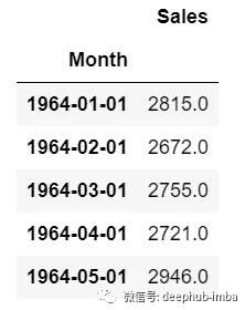
As we can see , There is only one column , Therefore, the upcoming future value will only depend on its previous value .

But in the case of multivariate time series data , There will be different types of eigenvalues and the target data will depend on these characteristics .

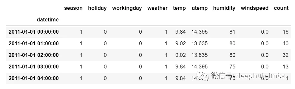
As you can see in the picture , In multivariate variables, there will be multiple columns to predict the target value .（ Above picture “count” For the target ）

In the data above ,count Not only depends on its previous value , It also depends on other characteristics . therefore , To predict the coming count value , We must consider all columns including the target column to predict the target value .

One thing to keep in mind when performing multivariate time series analysis , We need to use multiple features to predict the current goal , Let's take an example to understand ：

During the training , If we use 5 Column [feature1, feature2, feature3, feature4, target] To train the model , We need to provide... For the upcoming forecast day 4 Column [feature1, feature2, feature3, feature4].

LSTM

We do not intend to discuss in detail LSTM. So just provide some simple descriptions , If you are right about LSTM I don't know much about , You can refer to our previous articles .

LSTM It's basically a cyclic neural network , Ability to handle long-term dependencies .

Suppose you are watching a movie . So when anything happens in the movie , You already know what happened before , And it's understandable that new things happen because of what happened in the past .RNN It works the same way , They remember past information and use it to process current input .RNN The problem is , Because the gradient disappears , They cannot remember long-term dependencies . Therefore, in order to avoid the problem of long-term dependence lstm.

Now we discuss time series prediction and LSTM Theoretical part . Let's start coding .

Let's first import the libraries needed for forecasting ：

Load data , And check the output ：

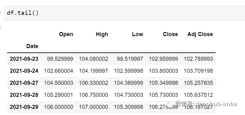
Now let's take a moment to look at the data ：csv The file contains Google from 2001-01-25 To 2021-09-29 Stock data for , The data is based on the frequency of days .

[ If you like , You can convert the frequency to “B”[ Working day ] or “D”, Because we don't use dates , I just keep it as it is .]

Here we try to predict “Open” The future value of the column , therefore “Open” It's the target column here .

Let's look at the shape of the data ：

Now let's do the training test . We can't mess up the data here , Because it must be sequential in the time series .

You can notice that the data range is very large , And they are not scaled in the same range , So in order to avoid prediction errors , Let's start with MinMaxScaler Scaling data .( You can also use StandardScaler)

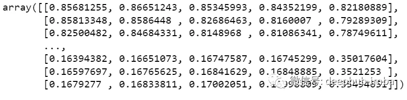
Split data into X and Y, This is the most important part , Read each step correctly .

Let's see what's done in the code above ：

N_past Is the number of steps we will look at in the past when predicting the next target value .

Use here 30, It means that the past 30 It's worth ( All features including target Columns ) To predict the 31 Target value .

therefore , stay trainX We will have all the eigenvalues , And in the trainY We only have the target value .

Let's break it down for Every part of the cycle ：

For training ,dataset = df_for_training_scaled, n_past=30

When i= 30：

from n_past The starting range is 30, So the first data range will be -[30 - 30,30,0:5] amount to [0:30,0:5]

So in dataX In the list ,df_for_training_scaled[0:30,0:5] The array will appear for the first time .

Now? , dataY.append(df_for_training_scaled[i,0])

i = 30, So it will only take the first 30 The line open( Because in the forecast , We just need open Column , So the column range is only 0, Express open Column ).

For the first time in dataY Store... In the list df_for_training_scaled[30,0] value .

They include 5 Before column 30 Rows are stored in dataX in , Only open In the column 31 Rows are stored in dataY in . Then we will dataX and dataY List to array , They are in array format LSTM Training in .

Let's look at the shape .

4132 yes trainX The total number of arrays available in , Each array has a total of 30 Row sum 5 Column , At the end of each array trainY in , We all have the next target value to train the model .

Let's look at the inclusion from trainX Of (30,5) One of the arrays of data and trainX Array of trainY value ：

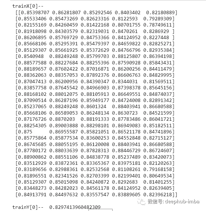
If you look at trainX[1] value , You will find that it is related to trainX[0] The data in is the same （ Except for the first column ）, Because we'll see before 30 To predict the second 31 Column , After the first prediction, it will automatically move To the first 2 Column and remove the next 30 Value to predict the next target value .

Let's explain all this in a simple format ：

like this , Each data will be saved in trainX and trainY in .

Now let's train the model , I use girdsearchCV Make some super parameter adjustments to find the basic model .

If you want to make more super parameter adjustments for your model , You can also add more layers . However, if the data set is very large, it is recommended to add LSTM Period and unit in the model .

At the first LSTM The input shape seen in the layer is (30,5). It comes from trainX shape .

Now let's fit the model to trainX and trainY In the data .

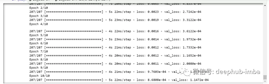
Due to the super parameter search , So it will take some time to run .

You can see that the loss will be reduced like this ：

Now let's check the best parameters of the model .

Save the best model in my_model variable .

Now you can test the model with the test data set .

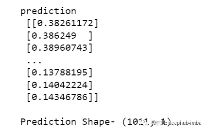
testY and prediction It's the same length . Now we can put testY Compare with the forecast .

But we scaled the data from the beginning , So first we have to do some inverse scaling process .

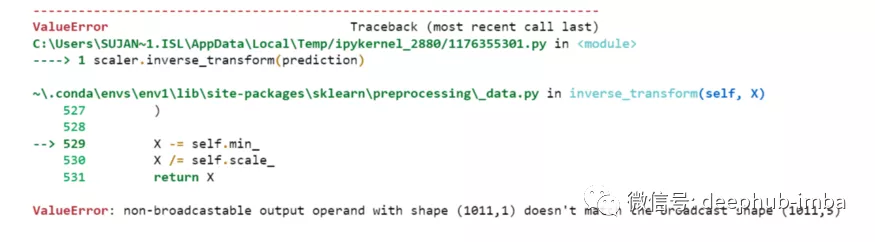
Wrong report , This is because when scaling data , We have... In each line 5 Column , Now we only have 1 Column is the target column .

So we have to change the shape to use inverse_transform：

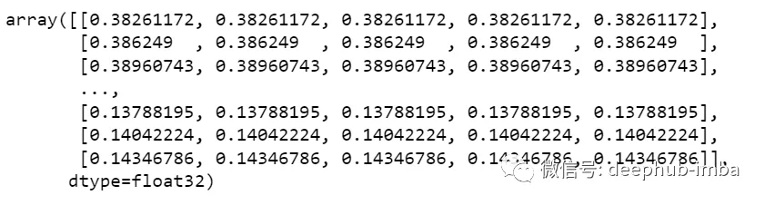
5 Column values are similar , It just copies a single forecast column 4 Time . So now we have 5 Column with the same value .

So you can use it inverse_transform function .

But the first column after inverse transformation is what we need , So we used... At the end → [:,0].

Now put this pred Value and testY Compare , however testY It's also scaled , You also need to use the same code as above for inverse transformation .

Now let's look at the predicted value and the original value ：

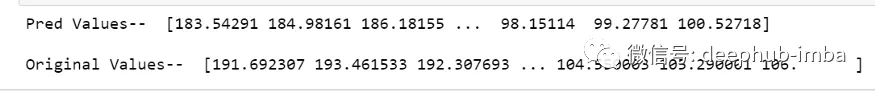
Finally, draw a diagram to compare our pred And raw data .

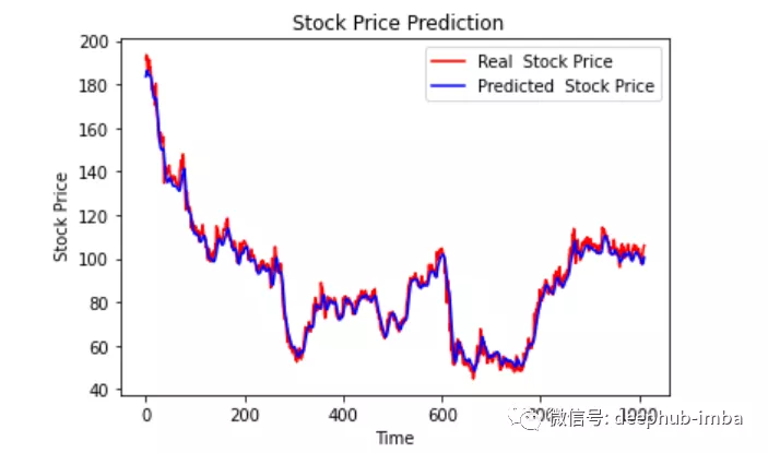
It looks good , up to now , We trained the model and checked the model with test values . Now let's predict some future values .

From the main df Get the last... We loaded at the beginning in the dataset 30 It's worth [ Why 30？ Because this is the number of past values we want , To predict the 31 It's worth ]

You can see that there are target Columns （“Open”） All columns including . Now let's predict the future 30 It's worth .

In multivariate time series prediction , You need to predict a single column by using different features , So we need to use eigenvalues when making predictions （ Except for the target column ） To make an upcoming forecast .

Here we need “High”、“Low”、“Close”、“Adj Close” Column's upcoming 30 A value for “Open” Column to predict .

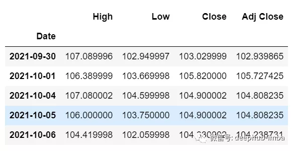
To eliminate “Open” After column , The following operations need to be done before using the model for prediction ：

Scaling data , Because deleted ‘Open’ Column , Before scaling it , Add a value that all values are “0” Of Open Column .

After zooming , In the future data “Open” Replace the column value with “nan”

Now attach 30 Days old value and 30 Tianxin value （ And finally 30 individual “ open ” The value is nan）

full_df   The shape is (60,5), Finally, the first column has 30 individual nan value .

To make a prediction, you must use... Again for loop , We're splitting trainX and trainY The data in . But this time we only have X, No, Y value .

For the first prediction , There is the former 30 It's worth , When for When the loop runs for the first time, it checks before 30 Value and predict the 31 individual “Open” data .

When the second for The loop will try to run , It will skip the first line and try to get the next 30 It's worth [1:31] . An error will be reported here because Open The last row of the column is “nan”, So you need to replace... With predictions every time “nan”.

Finally, the prediction needs to be inversely transformed ：

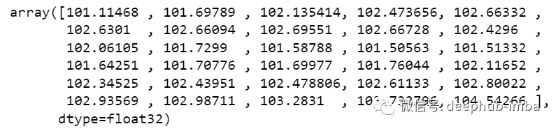
Such a complete process has run through .

This is about Python Use LSTM That's all for the detailed article on realizing sales forecast , More about Python LSTM Please search the previous articles of SDN or continue to browse the relevant articles below. I hope you will support SDN more in the future ！