大家可以關注知乎或微信公眾號的share16,我們也會同步更新此文章.
Disease prediction can often benefit from historical data mining of patients' medical records,Many valuable discoveries are often made in the modeling and analysis of structured data.Prediction and analysis through structured data,To determine whether a patient will develop acute liver failure.
this dataset,包含6000名20Adults over the age of 12008-2009和2014-2015of the two investigations.The data was collected from’JPAC Center for Health Diagnosis and Control‘所做的,A nationwide survey of adults:Research through professional visits,The dataset covers a wide range of population information and their health status,Sourced from direct interviews、Physical examination and blood sample examination(訓練集的比例為70%,測試集的比例為30%).
點此下載數據集
This question is to predict whether a patient will develop acute liver failure,結果只有0-1兩種可能,所以我們可以采用K近鄰算法、樸素貝葉斯、Logistic regression and decision trees are several algorithms.
補充:Automated parameter tuning,It can greatly reduce workload and improve work efficiency.Two commonly used parameter tuning methods are brute force search and random search.
查重 * 缺失值處理 * 分類變量(such as age segmentation) * Code categorical variables as dummy indicator variables(pd.get_dummies)等,詳見文章’機器學習(一)‘的第2.1節內容.
import numpy as np
import pandas as pd
from pyecharts.charts import *
import pyecharts.options as opts
from pyecharts.commons.utils import JsCode
from sklearn.model_selection import train_test_split,cross_val_score
from sklearn.linear_model import LogisticRegression
from sklearn.tree import DecisionTreeClassifier
from sklearn.naive_bayes import BernoulliNB
from sklearn.metrics import roc_auc_score
X = pd.read_csv('/XXXXXX/訓練集.csv')
Y = pd.read_csv('/XXXXXX/測試集.csv')
''' 修改列名 '''
x_cols,y_cols = [],[]
for i in X.columns.to_list():
if '\u2028' in i:
x_cols.append(i.split('\u2028')[1])
elif '\n' in i:
x_cols.append(i.split('\n')[1])
else:
x_cols.append(i)
for i in Y.columns.to_list():
if '\u2028' in i:
y_cols.append(i.split('\u2028')[1])
elif '\n' in i:
y_cols.append(i.split('\n')[1])
else:
y_cols.append(i)
X.columns = x_cols
Y.columns = y_cols
''' 填充缺失值 '''
x_name = X.isna().sum()[X.isna().sum()>0].index.to_list()
y_name = Y.isna().sum()[Y.isna().sum()>0].index.to_list()
X[x_name] = X[x_name].fillna(X[x_name].mean())
Y[y_name] = Y[y_name].fillna(Y[y_name].mean())
''' 分類變量 '''
X['Age'] = pd.cut(X.年齡,bins=[19,30,41,52,63,74,85],\
labels=['(19,30]','(30,41]','(41,52]','(52,63]','(63,74]','(74,85]'])
Y['Age'] = pd.cut(Y.年齡,bins=[19,30,41,52,63,74,85],\
labels=['(19,30]','(30,41]','(41,52]','(52,63]','(63,74]','(74,85]'])
''' 劃分數據集 '''
x_new = pd.get_dummies(X,columns=['Age','性別','區域','護理來源']).drop('年齡',axis=1)
x_0 = x_new.drop(columns=['id','ALF'],axis=1)
y_0 = x_new[['id','ALF']]
x_train,x_test,y_train,y_test = train_test_split(x_0,y_0,test_size=0.3,random_state=2022)
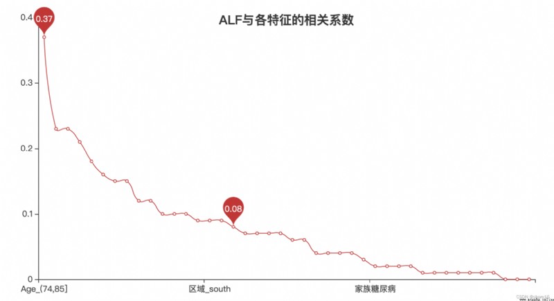
''' 相關系數 '''
r = abs(x_new.corr().round(2).ALF).sort_values(ascending=False).drop('id')
r_name = list(r.index)
l = Line()
l.add_xaxis(list(r.index)[1:])
l.add_yaxis('',list(r)[1:],is_smooth=True,label_opts=opts.LabelOpts(is_show=False),
markpoint_opts=opts.MarkPointOpts(data=[opts.MarkPointItem(type_='max',name='最大值'),\
opts.MarkPointItem(type_='average',name='平均值')]))
l.set_global_opts(title_opts=opts.TitleOpts('ALFCorrelation coefficients with each feature',pos_top='10%',pos_left='center'))
l.render_notebook()
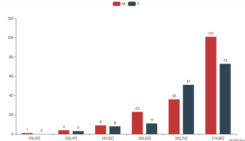
a = X[['id','Age','區域','性別','肝炎','高血壓','慢性疲勞','PVD','糖尿病','ALF']].round(2)
a_0 = a.groupby(['ALF','性別']).id.agg('count')
a_1 = a.groupby(['ALF','Age']).id.agg('count')
a_2 = a.groupby(['ALF','區域']).id.agg('count')
a_3 = a.groupby(['ALF','肝炎']).id.agg('count')
a_4 = a.groupby(['ALF','高血壓']).id.agg('count')
a_5 = a.groupby(['ALF','慢性疲勞']).id.agg('count')
a_6 = a.groupby(['ALF','PVD']).id.agg('count')
a_7 = a.groupby(['ALF','糖尿病']).id.agg('count')
a_11 = (a_1.loc[1,:]/a_1.reset_index().groupby('Age').id.agg('sum')*100).round(2).reset_index()
a_21 = (a_2.loc[1,:]/a_2.reset_index().groupby('區域').id.agg('sum')*100).round(2).reset_index()
a_31 = (a_3.loc[1,:]/a_3.reset_index().groupby('肝炎').id.agg('sum')*100).round(2).fillna(0)
a_41 = (a_4.loc[1,:]/a_4.reset_index().groupby('高血壓').id.agg('sum')*100).round(2).fillna(0)
a_51 = (a_5.loc[1,:]/a_5.reset_index().groupby('慢性疲勞').id.agg('sum')*100).round(2).fillna(0)
a_61 = (a_6.loc[1,:]/a_6.reset_index().groupby('PVD').id.agg('sum')*100).round(2).fillna(0)
a_71 = (a_7.loc[1,:]/a_7.reset_index().groupby('糖尿病').id.agg('sum')*100).round(2).fillna(0)
''' 性別/年齡/區域與ALF '''
p1 = Bar()
p1.add_xaxis(list(a_11.Age))
p1.add_yaxis('',list(a_11.id),bar_width='20%',label_opts=opts.LabelOpts(formatter='{c}%'),
color=JsCode("""new echarts.graphic.LinearGradient(0,0,0,1,\ [{offset:0,color:'#9DFEEC'},{offset:1,color:'#08B6D4'}],false)"""))
p1.set_global_opts(xaxis_opts=opts.AxisOpts(axisline_opts=opts.AxisLineOpts(is_show=False),
axistick_opts=opts.AxisTickOpts(is_show=False)),
yaxis_opts=opts.AxisOpts(is_show=False),
title_opts=opts.TitleOpts(title='age ratio of patients',subtitle='注:The number of patients in a certain age group/the number of people in this age group',
pos_top='1%',pos_right='10%'))
p2 = Bar()
p2.add_xaxis(list(a_21.區域))
p2.add_yaxis('',list(a_21.id),bar_width='20%',label_opts=opts.LabelOpts(formatter='{c}%'))
p2.reversal_axis()
p2.set_global_opts(xaxis_opts=opts.AxisOpts(is_show=False),yaxis_opts=opts.AxisOpts(is_inverse=True),
title_opts=opts.TitleOpts(title='Patient area ratio',subtitle='注:number of patients in an area/the number of people in the area',
pos_bottom='1%',pos_left='10%'))
p3 = Pie()
p3.add('',list((a_0.loc[1,:]/a_0.reset_index().groupby('性別').id.agg('sum')*100).round(2).to_dict().items()),
radius=['20%','30%'],center=['15%','35%'],
label_opts=opts.LabelOpts(position='inside',formatter='{b}:{c}%'))
p3.set_global_opts(title_opts=opts.TitleOpts(title='ratio of male to female patients',subtitle='注:The number of patients of a certain gender/the number of people of that gender'),
legend_opts=opts.LegendOpts(pos_top='10%',pos_left='left'))
grid = Grid()
grid.add(p1,grid_opts=opts.GridOpts(pos_top='11%',pos_left='50%',pos_right='1%'))
grid.add(p2,grid_opts=opts.GridOpts(pos_top='50%',pos_bottom='10%',pos_left='5%'))
grid.add(p3,grid_opts=opts.GridOpts(pos_top='11%',pos_left='1%'))
grid.render_notebook()
性別/年齡/區域與ALF的圖表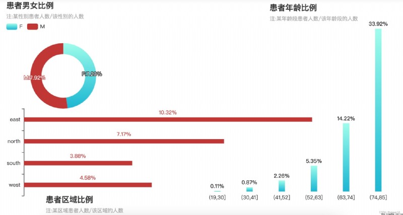
p4 = Pie()
p4.add('',list(a_31.to_dict().items()),radius=['10%','20%'],center=['15%','35%'],rosetype='area',
label_opts=opts.LabelOpts(formatter='{b}:{c}%'))
p4.set_colors(['#254EDB','#2CA127','#DBC72A'])
p4.set_global_opts(title_opts=opts.TitleOpts(title='ALFThe proportion of patients with hepatitis',subtitle='注:患者人數/總人數'),
legend_opts=opts.LegendOpts(pos_top='10%',pos_left='left'))
p5 = Pie()
p5.add('',list(a_41.to_dict().items()),radius=['10%','20%'],center=['45%','35%'],rosetype='area',
label_opts=opts.LabelOpts(formatter='{b}:{c}%'))
p5.set_colors(['#254EDB','#2CA127','#DBC72A'])
p5.set_global_opts(title_opts=opts.TitleOpts(title='ALFThe proportion of patients with hypertension',pos_top='1%',pos_left='35%'),
legend_opts=opts.LegendOpts(pos_top='10%',pos_left='40%'))
p6 = Pie()
p6.add('',list(a_51.to_dict().items()),radius=['10%','20%'],center=['75%','35%'],rosetype='area',
label_opts=opts.LabelOpts(formatter='{b}:{c}%'))
p6.set_colors(['#254EDB','#2CA127','#DBC72A'])
p6.set_global_opts(title_opts=opts.TitleOpts(title='ALFThe proportion of patients with chronic fatigue',pos_top='1%',pos_left='65%'),
legend_opts=opts.LegendOpts(pos_top='10%',pos_left='70%'))
p7 = Pie()
p7.add('',list(a_61.to_dict().items()),radius=['10%','20%'],center=['25%','85%'],rosetype='area',
label_opts=opts.LabelOpts(formatter='{b}:{c}%'))
p7.set_colors(['#254EDB','#2CA127','#DBC72A'])
p7.set_global_opts(title_opts=opts.TitleOpts(title='ALF患者PVD比例',pos_top='65%',pos_left='15%'),
legend_opts=opts.LegendOpts(is_show=False))
p8 = Pie()
p8.add('',list(a_71.to_dict().items()),radius=['10%','20%'],center=['60%','85%'],rosetype='area',
label_opts=opts.LabelOpts(formatter='{b}:{c}%'))
p8.set_colors(['#254EDB','#2CA127','#DBC72A'])
p8.set_global_opts(title_opts=opts.TitleOpts(title='ALFThe proportion of patients with diabetes',pos_top='65%',pos_left='45%'),
legend_opts=opts.LegendOpts(is_show=False))
grid = Grid()
grid.add(p4,grid_opts=opts.GridOpts(pos_top='20%',pos_left='10%'))
grid.add(p5,grid_opts=opts.GridOpts(pos_top='20%',pos_left='10%'))
grid.add(p6,grid_opts=opts.GridOpts(pos_top='20%',pos_left='10%'))
grid.add(p7,grid_opts=opts.GridOpts(pos_top='20%',pos_left='10%'))
grid.add(p8,grid_opts=opts.GridOpts(pos_top='20%',pos_left='10%'))
grid.render_notebook()
肝炎/high blood pressure, etcALF的圖表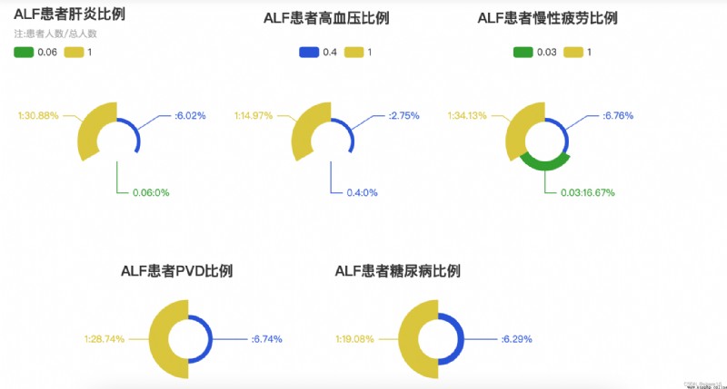
''' 交叉驗證,選出K個特征 '''
score = []
lr = LogisticRegression(solver='lbfgs',max_iter=6000)
for i in range(2,45):
s = cross_val_score(lr,x_train.loc[:,r_name[1:i]],y_train.iloc[:,1]).mean()
score.append(s)
k = range(2,45)[score.index(max(score))]
''' 暴力搜索-KNN '''
parameter = {
'n_neighbors':range(2,22)}
clf2 = GridSearchCV(KNeighborsClassifier(),parameter,cv=10)
clf2.fit(x_train.loc[:,r_name[1:k]],y_train.iloc[:,1])
print('Optimal parameter combination for brute force search:{}'.format(clf2.best_params_))
print('Optimal learner scoring for brute force search:',clf2.best_score_)
y_new = pd.get_dummies(Y,columns=['Age','性別','區域','護理來源']).drop('id',axis=1)
df = pd.DataFrame(data=clf2.predict(y_new.loc[:,r_name[1:k]]),index=Y.id,columns=['ALF']).reset_index()
#df.to_csv('/XXXXXX/df.csv',index=False)
#print('打印完成!')
df.ALF.sum()
運行結果:
Optimal parameter combination for brute force search:{‘n_neighbors’: 11}
Optimal learner scoring for brute force search:0.9231292517006804
Predicted number of patients:5
''' 貝葉斯-二項分布 '''
clf1 = BernoulliNB()
clf1.fit(x_train.loc[:,r_name[1:k]],y_train.iloc[:,1])
print('Bayesian score:',clf1.score(x_train.loc[:,r_name[1:k]],y_train.iloc[:,1]))
y_pre = clf1.predict(x_test.loc[:,r_name[1:k]])
print('貝葉斯auc值:',roc_auc_score(y_test.iloc[:,1],y_pre))
''' 預測新數據 '''
y_new = pd.get_dummies(Y,columns=['Age','性別','區域','護理來源']).drop('id',axis=1)
df = pd.DataFrame(data=clf1.predict(y_new.loc[:,r_name[1:k]]),index=Y.id,columns=['ALF']).reset_index()
#df.to_csv('/XXXXXX/df.csv',index=False)
#print('打印完成!')
df.ALF.sum()
運行結果:
Bayesian score:0.8826530612244898
貝葉斯auc值:0.7482117440969309
Predicted number of patients:201
''' 邏輯回歸 '''
lr.fit(x_train.loc[:,r_name[1:k]],y_train.iloc[:,1])
print('Logistic regression score:',lr.score(x_train.loc[:,r_name[1:k]],y_train.iloc[:,1]))
y_pre = lr.predict(x_test.loc[:,r_name[1:k]])
print('邏輯回歸auc值:',roc_auc_score(y_test.iloc[:,1],y_pre))
''' 預測新數據 '''
y_new = pd.get_dummies(Y,columns=['Age','性別','區域','護理來源']).drop('id',axis=1)
df = pd.DataFrame(data=lr.predict(y_new.loc[:,r_name[1:k]]),index=Y.id,columns=['ALF']).reset_index()
#df.to_csv('/XXXXXX/df.csv',index=False)
#print('打印完成!')
df.ALF.sum()
運行結果:
Logistic regression score:0.9258503401360544
邏輯回歸auc值:0.5595416225685194
Predicted number of patients:35
''' 決策樹 '''
clf = DecisionTreeClassifier()
clf.fit(x_train.loc[:,r_name[1:k]],y_train.iloc[:,1])
print('Decision tree score:',clf.score(x_train.loc[:,r_name[1:k]],y_train.iloc[:,1]))
y_pre = clf.predict(x_test.loc[:,r_name[1:k]])
print('決策樹auc值:',roc_auc_score(y_test.iloc[:,1],y_pre))
''' 預測新數據 '''
y_new = pd.get_dummies(Y,columns=['Age','性別','區域','護理來源']).drop('id',axis=1)
df = pd.DataFrame(data=clf.predict(y_new.loc[:,r_name[1:k]]),index=Y.id,columns=['ALF']).reset_index()
#df.to_csv('/XXXXXX/df.csv',index=False)
#print('打印完成!')
df.ALF.sum()
運行結果:
Decision tree score:1.0
決策樹auc值:0.6259534323564834
Predicted number of patients:141
It can be seen from the above,
① Female patients are slightly higher than males;
② 年齡越大,There is a higher likelihood of acute liver failure conditions,年紀在74~85歲之間,The probability of getting sick is up34%;
③ when people have hepatitis、慢性疲勞、PVD的狀況時,The probability of getting sick is up30%;
④ in this forecast,樸素貝葉斯-二項分布的auc值最好;
謝謝大家