Histogram is a statistical method for data , And organize the statistics into a series of implementation defined bin among . among bin It is a concept often used in histogram , It can be translated into “ Straight bar ” or “ Group spacing ”, Its value is the characteristic statistic calculated from the data , These data can be, for example, gradients 、 Direction 、 Color or any other feature .
Image histogram (Image Histogram) Is a histogram used to represent the brightness distribution in a digital image , The number of pixels of each luminance value in the image is plotted . In this histogram , The left side of the abscissa is the darker area . Therefore, the data in the histogram of a darker picture is mostly concentrated in the left and middle parts , And the whole is bright , Images with only a few shadows are the opposite .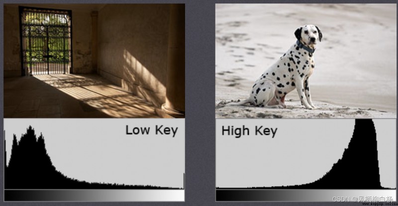
Be careful : Histogram is drawn according to gray image , Instead of color images . Suppose there is information about an image ( Gray value 0-255), The range of known numbers includes 256 It's worth , Therefore, this range can be divided into sub regions according to certain laws ( That is to say bins). Such as :
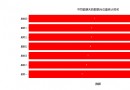
Then count each bin(i) The number of pixels . You can see the following ( among x Axis representation bin,y The axis represents each bin The number of pixels in ):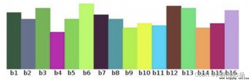
Here we need to pay attention to some technical terms in histogram description :
dims: Number of features to be counted , In the above example ,dims=1, Because it only represents the gray value
bins: The number of subsegments per feature space , It can be translated into “ Straight bar ” or “ Group spacing ”, In the example above ,bins=16
range: The value range of the feature to be counted . In the example above ,range = [0,255]
The significance of histogram :
Histogram is a graphical representation of the intensity distribution of pixels in an image
It counts the number of pixels per intensity value
The histograms of different images may be the same .
We usually use opencv Statistical histogram , And use matplotlib Draw it out .
API:
cv2.calcHist(images,channels,mask,histSize,ranges[,hist[,accumulate]])
Parameters :
images: Original image . When you pass in a function, you should use square brackets [] Cover up , for example :[img].
channels: If the input image is a grayscale image , Its value is [0]; If it's a color image , The parameter passed in can be [0],[1],[2] They correspond to channels B,G,R.
mask: mask image . To count the histogram of the whole image, set it to None. But if you want to count the histogram of a part of the image , You need to make a mask image , And use it .( There are examples later )
histSize:BIN Number of . It should also be enclosed in square brackets , for example :[256].
ranges: Pixel value range , Usually it is [0,256]
Code example :
import numpy as np
import cv2 as cv
from matplotlib import pyplot as plt
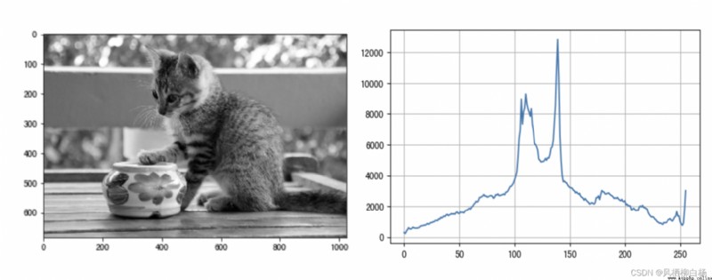
# 1 Read directly in the form of gray image
img = cv.imread('./image/cat.jpeg',0)
# 2 Statistical grayscale image
histr = cv.calcHist([img],[0],None,[256],[0,256])
# 3 Draw grayscale
plt.figure(figsize=(10,6),dpi=100)
plt.plot(histr)
plt.grid()
plt.show()
The mask is used with the selected image 、 Graphics or objects , Occlude the image to be processed , To control the area of image processing .
In digital image processing , We usually use a two-dimensional matrix array for masking . The mask is made of 0 and 1 Make up a binary image , The mask image is used to mask the image to be processed , among 1 The region of values is processed ,0 The value area is masked , Not deal with .
The main purpose of the mask is :
1、 Extract the region of interest : The image to be processed is processed with a pre made region of interest mask ” And “ operation , Get the ROI image , The image value in the region of interest remains the same , The out of area image values are 0.
2、 Shielding effect : Mask some areas of the image , Make it not participate in processing or calculation of processing parameters , Or only deal with or count the shielding area .
3、 Structural feature extraction : The similarity variable or image matching method is used to detect and extract the structural features similar to the mask in the image .
4、 Special shape image making
Mask on Remote sensing images More used in processing , When extracting roads or rivers 、 Or a house , The image is pixel filtered through a mask matrix , Then highlight the features or signs we need .
We use cv.calcHist() To find the histogram of the complete image . If you want to find the histogram of some areas of the image , Just create a white mask image on the area where you want to find the histogram , Otherwise, create black , Then use it as a mask mask Just pass it on .
Code example :
import numpy as np
import cv2 as cv
from matplotlib import pyplot as plt
# 1. Read directly in the form of gray image
img = cv.imread('./image/cat.jpeg',0)
# 2. Create a mask
mask = np.zeros(img.shape[:2], np.uint8)
mask[400:650, 200:500] = 255
# 3. Mask
masked_img = cv.bitwise_and(img,img,mask = mask)
# 4. Count the gray image of the image after the mask
mask_histr = cv.calcHist([img],[0],mask,[256],[1,256])
# 5. Image display
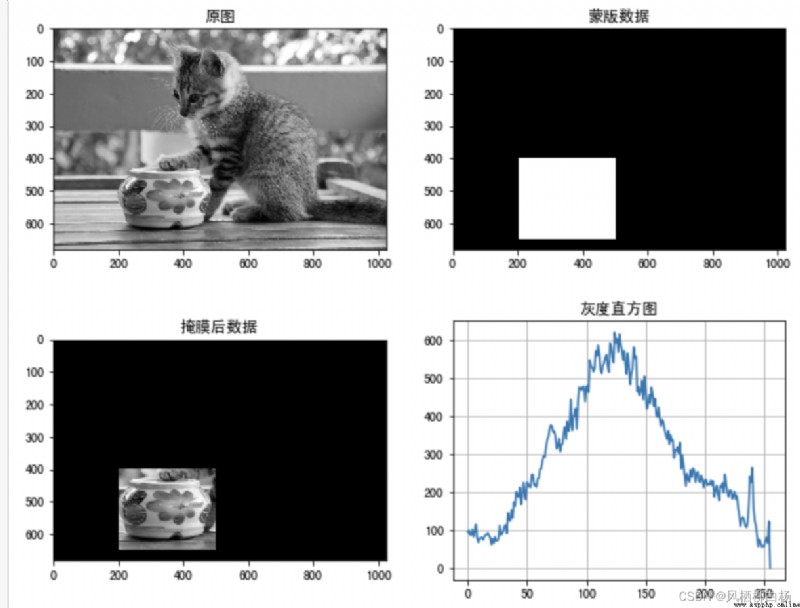
fig,axes=plt.subplots(nrows=2,ncols=2,figsize=(10,8))
axes[0,0].imshow(img,cmap=plt.cm.gray)
axes[0,0].set_title(" Original picture ")
axes[0,1].imshow(mask,cmap=plt.cm.gray)
axes[0,1].set_title(" Mask data ")
axes[1,0].imshow(masked_img,cmap=plt.cm.gray)
axes[1,0].set_title(" Post mask data ")
axes[1,1].plot(mask_histr)
axes[1,1].grid()
axes[1,1].set_title(" Gray histogram ")
plt.show()
Imagine , What if the pixel values of most pixels in an image are concentrated in a small gray value range ? If an image is bright as a whole , The number of values of all pixel values should be very high . So you should stretch its histogram horizontally ( Here's the picture ), The distribution range of image pixel values can be expanded , Improve the contrast of the image , This is what histogram equalization should do .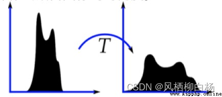
“ Histogram equalization ” It is to change the gray histogram of the original image from a relatively concentrated gray interval to a distribution in a wider gray range . Histogram equalization is the nonlinear stretching of the image , Reassign image pixel values , Make the number of pixels in a certain gray range approximately the same .
This method improves the overall contrast of the image , Especially when the pixel value distribution of useful data is close , stay X Optical images are widely used , It can improve the display of skeleton structure , In addition, it can better highlight details in overexposed or underexposed images .
Use opencv Histogram statistics , It uses :
API:
dst = cv.equalizeHist(img)
Parameters :
img: Grayscale image
return :
dst : The result of equalization
Code example :
import numpy as np
import cv2 as cv
from matplotlib import pyplot as plt
# 1. Read directly in the form of gray image
img = cv.imread('./image/cat.jpeg',0)
# 2. Equalization treatment
dst = cv.equalizeHist(img)
# 3. Result display
fig,axes=plt.subplots(nrows=2,ncols=2,figsize=(10,8),dpi=100)
axes[0].imshow(img,cmap=plt.cm.gray)
axes[0].set_title(" Original picture ")
axes[1].imshow(dst,cmap=plt.cm.gray)
axes[1].set_title(" The result after equalization ")
plt.show()
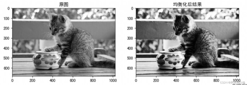
Histogram equalization above , What we consider is the global contrast of the image . Indeed, after histogram equalization , The contrast of the picture background has been changed , It's too dark here in the cat's legs , We lost a lot of information , So in many cases , It doesn't work well . As shown in the figure below , Compare the picture of the statue in the next two images , We lost a lot of information because it was too bright .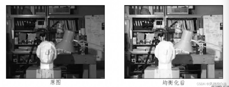
To solve this problem , Adaptive histogram equalization is needed . here , The whole image will be divided into many small pieces , These small pieces are called “tiles”( stay OpenCV in tiles Of The default size is 8x8), Then histogram equalization is performed for each small block . So in every area , The histogram will be concentrated in a small area ). If there is noise , The noise will be amplified . To avoid this, use contrast limits . For each small piece , If... In the histogram bin If you exceed the upper limit of contrast , Just put The pixels are evenly distributed to other areas bins in , Then histogram equalization .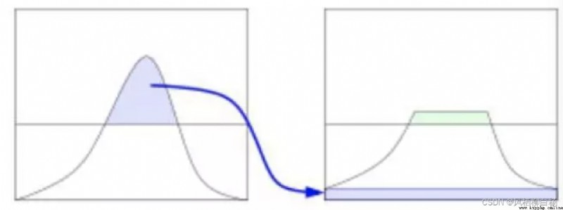 Last , in order to Remove the boundary between each small block , Then use bilinear difference , Splice each small piece .
API:
cv.createCLAHE(clipLimit, tileGridSize)
Parameters :
clipLimit: Contrast limit , The default is 40
tileGridSize: The size of the blocks , The default is 8*88∗8
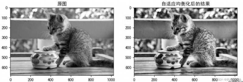
Code example
import numpy as np
import cv2 as cv
# 1. Read the image in the form of grayscale image
img = cv.imread('./image/cat.jpeg',0)
# 2. Create an adaptive equalization object , And applied to image
clahe = cv.createCLAHE(clipLimit=2.0, tileGridSize=(8,8))
cl1 = clahe.apply(img)
# 3. Image display
fig,axes=plt.subplots(nrows=1,ncols=2,figsize=(10,8),dpi=100)
axes[0].imshow(img,cmap=plt.cm.gray)
axes[0].set_title(" Original picture ")
axes[1].imshow(cl1,cmap=plt.cm.gray)
axes[1].set_title(" The result of adaptive equalization ")
plt.show()
Histogram is a graphical representation of the intensity distribution of pixels in an image .
It counts the number of pixels per intensity value .
The histograms of different images may be the same
cv.calcHist(images,channels,mask,histSize,ranges [,hist [,accumulate]])
I haven't really understood this part yet , Understand later , I will optimize this place again .