因為訓練單詞嵌入在計算上非常耗時耗力,所以大多數ML練習者都會加載一組經過預先訓練的嵌入。
完成此任務後,你將能夠:
import numpy as np
from w2v_utils import *
Using TensorFlow backend.
接下來,讓我們加載單詞向量。對於此作業,我們將使用50維GloVe向量表示單詞。運行以下單元格以加載word_to_vec_map。
words, word_to_vec_map = read_glove_vecs('data/glove.6B.50d.txt')
你已加載:
words:詞匯表中的單詞集。word_to_vec_map:將單詞映射到其CloVe向量表示的字典上。你已經看到,單向向量不能很好地說明相似的單詞。GloVe向量提供有關單個單詞含義的更多有用信息。現在讓我們看看如何使用GloVe向量確定兩個單詞的相似程度。
要測量兩個單詞的相似程度,我們需要一種方法來測量兩個單詞的兩個嵌入向量之間的相似度。給定兩個向量 u u u和 v v v,余弦相似度定義如下:
CosineSimilarity(u, v) = u ⋅ v ∣ ∣ u ∣ ∣ 2 ∣ ∣ v ∣ ∣ 2 = c o s ( θ ) (1) \text{CosineSimilarity(u, v)} = \frac {u \cdot v} {||u||_2 ||v||_2} = cos(\theta) \tag{1} CosineSimilarity(u, v)=∣∣u∣∣2∣∣v∣∣2u⋅v=cos(θ)(1)
其中 u ⋅ v u \cdot v u⋅v是兩個向量的點積(或內積), ∣ ∣ u ∣ ∣ 2 ||u||_2 ∣∣u∣∣2是向量 u u u的范數(或長度),而 θ \theta θ是 u u u和 v v v之間的夾角。這種相似性取決於 u u u和 v v v之間的角度。如果 u u u和 v v v非常相似,他們的余弦相似度將接近1;如果它們不相似,則余弦相似度將取較小的值。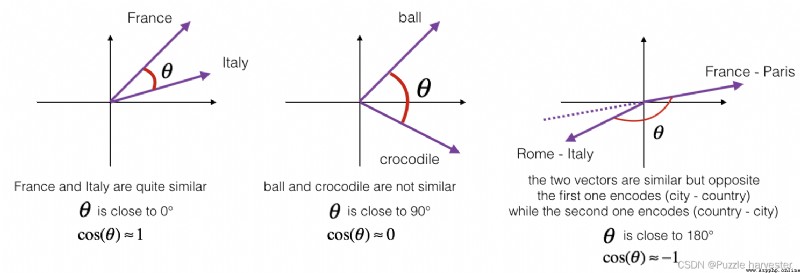
圖1:兩個向量之間的夾角余弦表示它們的相似度
練習:實現函數cosine_similarity()以評估單詞向量之間的相似性。
提醒: u u u的范數定義為$ ||u||2 = \sqrt{\sum{i=1}^{n} u_i^2}$。
def cosine_similarity(u, v):
""" u與v的余弦相似度反映了u與v的相似程度 參數: u -- 維度為(n,)的詞向量 v -- 維度為(n,)的詞向量 返回: cosine_similarity -- 由上面公式定義的u和v之間的余弦相似度。 """
distance = 0
# 計算u與v的內積
dot = np.dot(u, v)
#計算u的L2范數
norm_u = np.sqrt(np.sum(np.power(u, 2)))
#計算v的L2范數
norm_v = np.sqrt(np.sum(np.power(v, 2)))
# 根據公式1計算余弦相似度
cosine_similarity = np.divide(dot, norm_u * norm_v)
return cosine_similarity
father = word_to_vec_map["father"]
mother = word_to_vec_map["mother"]
ball = word_to_vec_map["ball"]
crocodile = word_to_vec_map["crocodile"]
france = word_to_vec_map["france"]
italy = word_to_vec_map["italy"]
paris = word_to_vec_map["paris"]
rome = word_to_vec_map["rome"]
print("cosine_similarity(father, mother) = ", cosine_similarity(father, mother))
print("cosine_similarity(ball, crocodile) = ",cosine_similarity(ball, crocodile))
print("cosine_similarity(france - paris, rome - italy) = ",cosine_similarity(france - paris, rome - italy))
cosine_similarity(father, mother) = 0.8909038442893615
cosine_similarity(ball, crocodile) = 0.2743924626137942
cosine_similarity(france - paris, rome - italy) = -0.6751479308174201
獲得正確的預期輸出後,請隨時修改輸入並測量其他詞對之間的余弦相似度!圍繞其他輸入的余弦相似性進行操作將使你對單詞向量的表征有更好的了解。
在類比任務中,我們完成句子"a is to b as c is to __"。 一個例子是’man is to woman as king is to queen'。 詳細地說,我們試圖找到一個單詞d,以使關聯的單詞向量 e a , e b , e c , e d e_a, e_b, e_c, e_d ea,eb,ec,ed通過以下方式相關: e b − e a ≈ e d − e c e_b - e_a \approx e_d - e_c eb−ea≈ed−ec。我們將使用余弦相似性來衡量 e b − e a e_b - e_a eb−ea和 e d − e c e_d - e_c ed−ec之間的相似性。
練習:完成以下代碼即可執行單詞類比!
def complete_analogy(word_a, word_b, word_c, word_to_vec_map):
""" 解決“A與B相比就類似於C與____相比一樣”之類的問題 參數: word_a -- 一個字符串類型的詞 word_b -- 一個字符串類型的詞 word_c -- 一個字符串類型的詞 word_to_vec_map -- 字典類型,單詞到GloVe向量的映射 返回: best_word -- 滿足(v_b - v_a) 最接近 (v_best_word - v_c) 的詞 """
# 把單詞轉換為小寫
word_a, word_b, word_c = word_a.lower(), word_b.lower(), word_c.lower()
# 獲取對應單詞的詞向量
e_a, e_b, e_c = word_to_vec_map[word_a], word_to_vec_map[word_b], word_to_vec_map[word_c]
# 獲取全部的單詞
words = word_to_vec_map.keys()
# 將max_cosine_sim初始化為一個比較大的負數
max_cosine_sim = -100
best_word = None
# 遍歷整個數據集
for word in words:
# 要避免匹配到輸入的數據
if word in [word_a, word_b, word_c]:
continue
# 計算余弦相似度
cosine_sim = cosine_similarity((e_b - e_a), (word_to_vec_map[word] - e_c))
if cosine_sim > max_cosine_sim:
max_cosine_sim = cosine_sim
best_word = word
return best_word
triads_to_try = [('italy', 'italian', 'spain'), ('india', 'delhi', 'japan'), ('man', 'woman', 'boy'), ('small', 'smaller', 'large')]
for triad in triads_to_try:
print ('{} -> {} <====> {} -> {}'.format( *triad, complete_analogy(*triad,word_to_vec_map)))
italy -> italian <====> spain -> spanish
india -> delhi <====> japan -> tokyo
man -> woman <====> boy -> girl
small -> smaller <====> large -> larger
你可以隨意地去更改上面的詞匯,看看能否拿到自己期望的輸出,你也可以試試能不能讓程序出一點小錯呢?比如:small -> smaller <===> big -> ? ,自己試試呗~
triads_to_try = [('small', 'smaller', 'big')]
for triad in triads_to_try:
print ('{} -> {} <====> {} -> {}'.format( *triad, complete_analogy(*triad,word_to_vec_map)))
small -> smaller <====> big -> competitors
以下是你應記住的要點:
在下面的練習中,你將研究可嵌入詞嵌入的性別偏見,並探索減少偏見的算法。除了了解去偏斜的主題外,本練習還將幫助你磨清直覺,了解單詞向量在做什麼。本節涉及一些線性代數,盡管即使你不擅長線性代數,你也可以完成它,我們鼓勵你嘗試一下。
首先讓我們看看GloVe詞嵌入與性別之間的關系。你將首先計算向量 g = e w o m a n − e m a n g = e_{woman}-e_{man} g=ewoman−eman,其中 e w o m a n e_{woman} ewoman表示與單詞woman對應的單詞向量,而 e m a n e_{man} eman則與單詞對應與單詞man對應的向量。所得向量 g g g大致編碼“性別”的概念。(如果你計算 g 1 = e m o t h e r − e f a t h e r g_1 = e_{mother}-e_{father} g1=emother−efather, g 2 = e g i r l − e b o y g_2 = e_{girl}-e_{boy} g2=egirl−eboy等,並對其進行平均,則可能會得到更准確的表示。但是僅使用 e w o m a n − e m a n e_{woman}-e_{man} ewoman−eman會給你足夠好的結果。)
g = word_to_vec_map['woman'] - word_to_vec_map['man']
print(g)
[-0.087144 0.2182 -0.40986 -0.03922 -0.1032 0.94165
-0.06042 0.32988 0.46144 -0.35962 0.31102 -0.86824
0.96006 0.01073 0.24337 0.08193 -1.02722 -0.21122
0.695044 -0.00222 0.29106 0.5053 -0.099454 0.40445
0.30181 0.1355 -0.0606 -0.07131 -0.19245 -0.06115
-0.3204 0.07165 -0.13337 -0.25068714 -0.14293 -0.224957
-0.149 0.048882 0.12191 -0.27362 -0.165476 -0.20426
0.54376 -0.271425 -0.10245 -0.32108 0.2516 -0.33455
-0.04371 0.01258 ]
現在,你將考慮一下不同單詞 g g g的余弦相似度。考慮相似性的正值與余弦相似性的負值意味著什麼。
print ('List of names and their similarities with constructed vector:')
# girls and boys name
name_list = ['john', 'marie', 'sophie', 'ronaldo', 'priya', 'rahul', 'danielle', 'reza', 'katy', 'yasmin']
for w in name_list:
print (w, cosine_similarity(word_to_vec_map[w], g))
List of names and their similarities with constructed vector:
john -0.23163356145973724
marie 0.315597935396073
sophie 0.31868789859418784
ronaldo -0.31244796850329437
priya 0.17632041839009402
rahul -0.16915471039231716
danielle 0.24393299216283895
reza -0.07930429672199553
katy 0.2831068659572615
yasmin 0.23313857767928758
如你所見,女性名字與我們構造的向量 g g g的余弦相似度為正,而男性名字與余弦的相似度為負。這並不令人驚訝,結果似乎可以接受。
但是,讓我們嘗試其他一些話。
print('Other words and their similarities:')
word_list = ['lipstick', 'guns', 'science', 'arts', 'literature', 'warrior','doctor', 'tree', 'receptionist',
'technology', 'fashion', 'teacher', 'engineer', 'pilot', 'computer', 'singer']
for w in word_list:
print (w, cosine_similarity(word_to_vec_map[w], g))
Other words and their similarities:
lipstick 0.2769191625638267
guns -0.1888485567898898
science -0.06082906540929701
arts 0.008189312385880337
literature 0.06472504433459932
warrior -0.20920164641125288
doctor 0.11895289410935041
tree -0.07089399175478091
receptionist 0.33077941750593737
technology -0.13193732447554302
fashion 0.03563894625772699
teacher 0.17920923431825664
engineer -0.0803928049452407
pilot 0.0010764498991916937
computer -0.10330358873850498
singer 0.1850051813649629
你有什麼驚訝的地方嗎?令人驚訝的是,這些結果如何反映出某些不健康的性別定型觀念。例如,“computer"更接近 “man”,而"literature” 更接近"woman"。
我們將在下面看到如何使用Boliukbasi et al., 2016提出的算法來減少這些向量的偏差。注意,諸如 “actor”/“actress” 或者 “grandmother”/“grandfather"之類的詞對應保持性別特定,而諸如"receptionist” 或者"technology"之類的其他詞語應被中和,即與性別無關。消除偏見時,你將不得不區別對待這兩種類型的單詞。
下圖應幫助你直觀地了解中和的作用。如果你使用的是50維詞嵌入,則50維空間可以分為兩部分:偏移方向 g g g和其余49維,我們將其稱為 g ⊥ g_{\perp} g⊥。在線性代數中,我們說49維 g ⊥ g_{\perp} g⊥與 g g g垂直(或“正交”),這意味著它與 g g g成90度。中和步驟采用向量,例如 e r e c e p t i o n i s t e_{receptionist} ereceptionist,並沿 g g g的方向將分量清零,從而得到 e r e c e p t i o n i s t d e b i a s e d e_{receptionist}^{debiased} ereceptionistdebiased。
即使 g ⊥ g_{\perp} g⊥是49維的,鑒於我們可以在屏幕上繪制的內容的局限性,我們還是使用下面的1維軸對其進行說明。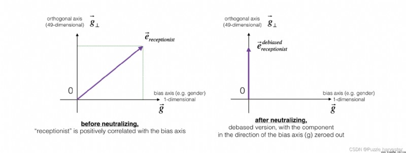
圖2:在應用中和操作之前和之後,代表"receptionist"的單詞向量。
練習:實現neutralize()以消除諸如"receptionist" 或 "scientist"之類的詞的偏見。給定嵌入 e e e的輸入,你可以使用以下公式來計算 e d e b i a s e d e^{debiased} edebiased:
e b i a s _ c o m p o n e n t = e ⋅ g ∣ ∣ g ∣ ∣ 2 2 ∗ g (2) e^{bias\_component} = \frac{e \cdot g}{||g||_2^2} * g\tag{2} ebias_component=∣∣g∣∣22e⋅g∗g(2)
e d e b i a s e d = e − e b i a s _ c o m p o n e n t (3) e^{debiased} = e - e^{bias\_component}\tag{3} edebiased=e−ebias_component(3)
如果你是線性代數方面的專家,則可以將 e b i a s _ c o m p o n e n t e^{bias\_component} ebias_component識別為 e e e在 g g g方向上的投影。如果你不是線性代數方面的專家,請不必為此擔心。
提醒:向量 u u u可分為兩部分:在向量軸 v B v_B vB上的投影和在與 v v v正交的軸上的投影:
u = u B + u ⊥ u = u_B + u_{\perp} u=uB+u⊥
其中: u B = u_B= uB= and u ⊥ = u − u B u_{\perp} =u - u_B u⊥=u−uB
def neutralize(word, g, word_to_vec_map):
""" 通過將“word”投影到與偏置軸正交的空間上,消除了“word”的偏差。 該函數確保“word”在性別的子空間中的值為0 參數: word -- 待消除偏差的字符串 g -- 維度為(50,),對應於偏置軸(如性別) word_to_vec_map -- 字典類型,單詞到GloVe向量的映射 返回: e_debiased -- 消除了偏差的向量。 """
# 根據word選擇對應的詞向量
e = word_to_vec_map[word]
# 根據公式2計算e_biascomponent
e_biascomponent = np.divide(np.dot(e, g), np.square(np.linalg.norm(g))) * g
# 根據公式3計算e_debiased
e_debiased = e - e_biascomponent
return e_debiased
e = "receptionist"
print("去偏差前{0}與g的余弦相似度為:{1}".format(e, cosine_similarity(word_to_vec_map["receptionist"], g)))
e_debiased = neutralize("receptionist", g, word_to_vec_map)
print("去偏差後{0}與g的余弦相似度為:{1}".format(e, cosine_similarity(e_debiased, g)))
去偏差前receptionist與g的余弦相似度為:0.33077941750593737
去偏差後receptionist與g的余弦相似度為:-2.099120994400013e-17
接下來,讓我們看一下如何將偏置也應用於單詞對,例如"actress"和"actor"。均衡僅應用與你希望通過性別屬性有所不同的單詞對。作為具體示例,假設"actress"比"actor"更接近"babysit"。通過將中和應用於"babysit",我們可以減少與"babysit"相關的性別刻板印象。但這仍然不能保證"actress"和"actor"與"babysit"等距,均衡算法負責這一點。
均衡背後的關鍵思想是確保一對特定單詞與49維 g ⊥ g_{\perp} g⊥等距。均衡步驟還確保了兩個均衡步驟現在與 e r e c e p t i o n i s t d e b i a s e d e_{receptionist}^{debiased} ereceptionistdebiased或與任何其他已中和的作品之間的距離相同。圖片中展示了均衡的工作方式: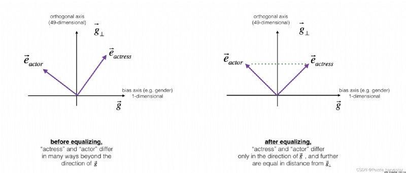
為此,線性代數的推導要復雜一些。(詳細信息請參見Bolukbasi et al., 2016)但其關鍵方程式是:
μ = e w 1 + e w 2 2 (4) \mu = \frac{e_{w1} + e_{w2}}{2}\tag{4} μ=2ew1+ew2(4)
KaTeX parse error: Expected 'EOF', got '_' at position 39: …cdot \text{bias_̲axis}}{||\text{…
μ ⊥ = μ − μ B (6) \mu_{\perp} = \mu - \mu_{B} \tag{6} μ⊥=μ−μB(6)
KaTeX parse error: Expected 'EOF', got '_' at position 42: …cdot \text{bias_̲axis}}{||\text{…
KaTeX parse error: Expected 'EOF', got '_' at position 42: …cdot \text{bias_̲axis}}{||\text{…
e w 1 B c o r r e c t e d = ∣ 1 − ∣ ∣ μ ⊥ ∣ ∣ 2 2 ∣ ∗ e w1B − μ B ∣ ( e w 1 − μ ⊥ ) − μ B ) ∣ (9) e_{w1B}^{corrected} = \sqrt{ |{1 - ||\mu_{\perp} ||^2_2} |} * \frac{e_{\text{w1B}} - \mu_B} {|(e_{w1} - \mu_{\perp}) - \mu_B)|} \tag{9} ew1Bcorrected=∣1−∣∣μ⊥∣∣22∣∗∣(ew1−μ⊥)−μB)∣ew1B−μB(9)
e w 2 B c o r r e c t e d = ∣ 1 − ∣ ∣ μ ⊥ ∣ ∣ 2 2 ∣ ∗ e w2B − μ B ∣ ( e w 2 − μ ⊥ ) − μ B ) ∣ (10) e_{w2B}^{corrected} = \sqrt{ |{1 - ||\mu_{\perp} ||^2_2} |} * \frac{e_{\text{w2B}} - \mu_B} {|(e_{w2} - \mu_{\perp}) - \mu_B)|} \tag{10} ew2Bcorrected=∣1−∣∣μ⊥∣∣22∣∗∣(ew2−μ⊥)−μB)∣ew2B−μB(10)
e 1 = e w 1 B c o r r e c t e d + μ ⊥ (11) e_1 = e_{w1B}^{corrected} + \mu_{\perp} \tag{11} e1=ew1Bcorrected+μ⊥(11)
e 2 = e w 2 B c o r r e c t e d + μ ⊥ (12) e_2 = e_{w2B}^{corrected} + \mu_{\perp} \tag{12} e2=ew2Bcorrected+μ⊥(12)
練習:實現以下函數。使用上面的等式來獲取單詞對的最終均等化形式。
def equalize(pair, bias_axis, word_to_vec_map):
""" 通過遵循上圖中所描述的均衡方法來消除性別偏差。 參數: pair -- 要消除性別偏差的詞組,比如 ("actress", "actor") bias_axis -- 維度為(50,),對應於偏置軸(如性別) word_to_vec_map -- 字典類型,單詞到GloVe向量的映射 返回: e_1 -- 第一個詞的詞向量 e_2 -- 第二個詞的詞向量 """
# 第1步:獲取詞向量
w1, w2 = pair
e_w1, e_w2 = word_to_vec_map[w1], word_to_vec_map[w2]
# 第2步:計算w1與w2的均值
mu = (e_w1 + e_w2) / 2.0
# 第3步:計算mu在偏置軸與正交軸上的投影
mu_B = np.divide(np.dot(mu, bias_axis), np.square(np.linalg.norm(bias_axis))) * bias_axis
mu_orth = mu - mu_B
# 第4步:使用公式7、8計算e_w1B 與 e_w2B
e_w1B = np.divide(np.dot(e_w1, bias_axis), np.square(np.linalg.norm(bias_axis))) * bias_axis
e_w2B = np.divide(np.dot(e_w2, bias_axis), np.square(np.linalg.norm(bias_axis))) * bias_axis
# 第5步:根據公式9、10調整e_w1B 與 e_w2B的偏置部分
corrected_e_w1B = np.sqrt(np.abs(1-np.square(np.linalg.norm(mu_orth)))) * np.divide(e_w1B-mu_B, np.abs(e_w1 - mu_orth - mu_B))
corrected_e_w2B = np.sqrt(np.abs(1-np.square(np.linalg.norm(mu_orth)))) * np.divide(e_w2B-mu_B, np.abs(e_w2 - mu_orth - mu_B))
# 第6步: 使e1和e2等於它們修正後的投影之和,從而消除偏差
e1 = corrected_e_w1B + mu_orth
e2 = corrected_e_w2B + mu_orth
return e1, e2
print("==========均衡校正前==========")
print("cosine_similarity(word_to_vec_map[\"man\"], gender) = ", cosine_similarity(word_to_vec_map["man"], g))
print("cosine_similarity(word_to_vec_map[\"woman\"], gender) = ", cosine_similarity(word_to_vec_map["woman"], g))
e1, e2 = equalize(("man", "woman"), g, word_to_vec_map)
print("\n==========均衡校正後==========")
print("cosine_similarity(e1, gender) = ", cosine_similarity(e1, g))
print("cosine_similarity(e2, gender) = ", cosine_similarity(e2, g))
==========均衡校正前==========
cosine_similarity(word_to_vec_map["man"], gender) = -0.11711095765336832
cosine_similarity(word_to_vec_map["woman"], gender) = 0.35666618846270376
==========均衡校正後==========
cosine_similarity(e1, gender) = -0.7165727525843935
cosine_similarity(e2, gender) = 0.7396596474928909
請隨意使用上方單元格中的輸入單詞,以將均衡應用於其他單詞對。
這些去偏置算法對於減少偏差非常有幫助,但並不完美,並且不能消除所有偏差痕跡。例如,該實現的一個缺點是僅使用單詞woman和man來定義偏差方向 g g g。如前所述,如果 g g g是通過計算 g 1 = e w o m a n − e m a n g_1 = e_{woman} - e_{man} g1=ewoman−eman; g 2 = e m o t h e r − e f a t h e r g_2 = e_{mother} - e_{father} g2=emother−efather; g 3 = e g i r l − e b o y g_3 = e_{girl} - e_{boy} g3=egirl−eboy等等來定義的,然後對它們進行平均,可以更好地估計50維單詞嵌入空間中的“性別”維度。也可以隨意使用這些變體。
 Python:difflib. Sequencematcher compares the text content and returns the difference part
Knowledge points applied :s=di
 Anaconda3-5.2.0+python3.6 steps and procedures for installing opencv-python3.4.1.15
Installation steps Directory :