This tutorial is designed to help students who have no foundation Fast grasp numpy Common functions of , Ensure the use of most daily scenes . It can be used as a prerequisite course for machine learning or deep learning , It can also be used as a quick reference manual .
It is worth mentioning that , There are many frameworks for deep learning API and numpy It comes down in one continuous line , so to speak numpy Play familiar , Several in-depth learning frameworks API Also learned . This article is the of the tutorial 「 The first part 」, Starting from the actual code application , Explained Numpy Create operations to statistics .

Open source project address :https://github.com/datawhalechina/powerful-numpy
notes :B There is a video tutorial explained by the author (B The number of people standing to watch is more than ten thousand ٩(๑>◡<๑)۶), Welcome to the account Two dimensional Datawhale Search for 「 Very hard Numpy」, Get a first-hand explanation .
Original tutorial Is the following : · Practical and high frequency API · Show the actual usage · Simple and direct Use explain : In content (1-5 individual ) Indicates the degree of importance , The more, the more important ;️ Indicates something that requires special attention Tips : There is no need to pay too much attention to API Details of various parameters , The usage provided in the tutorial is enough to cope with the overwhelming Most of the scenes , Follow up tutorials or more in-depth explorations as needed . Now let's officially begin to explain .
#  Import  library
import numpy as np
#  drawing tools
import matplotlib.pyplot as plt
This section focuses on the introduction array Creation and generation of . Why put this at the front ? There are two main reasons :
First , In the course of practical work , From time to time, we need to verify or check array dependent API Or interoperability . meanwhile , Sometimes in use sklearn,matplotlib,PyTorch,Tensorflow And other tools also need some simple data to experiment .
therefore , First learn how to get one quickly array There are many benefits . In this section, we mainly introduce the following common creation methods :
Use lists or tuples
Use arange
Use linspace/logspace
Use ones/zeros
Use random
Read from file
among , The most commonly used is linspace/logspace and random, The former is often used to draw coordinate axes , The latter is used to generate 「 Analog data 」. for instance , When we need to draw an image of a function ,X Often use linspace Generate , Then use the function formula to find Y, Again plot; When we need to construct some input ( such as X) Or intermediate input ( such as Embedding、hidden state) when ,random It will be very convenient .
Focus on mastery list Create a array that will do :np.array(list)
️ It should be noted that :「 data type 」. If you are careful enough , You can find the second set of codes below 2 The number is 「 decimal 」( notes :Python in 1. == 1.0), and array Is to ensure that each element type is the same , So I'll help you array Turn to one float The type of .
#  One  list
np.array([1,2,3])
array([1, 2, 3])
#  A two-dimensional ( Multidimensional similar )
#  Be careful , There is a decimal
np.array([[1, 2., 3], [4, 5, 6]])
array([[1., 2., 3.],
 [4., 5., 6.]])
#  You can also specify the data type
np.array([1, 2, 3], dtype=np.float16)
array([1., 2., 3.], dtype=float16)
#  If you specify  dtype, The value entered will be converted to the corresponding type , And it won't be rounded
lst = [
    [1, 2, 3],
    [4, 5, 6.8]
]
np.array(lst, dtype=np.int32)
array([[1, 2, 3],
 [4, 5, 6]], dtype=int32)
#  One  tuple
np.array((1.1, 2.2))
array([1.1, 2.2])
# tuple, It's usually used  list  Just fine , No need to use  tuple
np.array([(1.1, 2.2, 3.3), (4.4, 5.5, 6.6)])
array([[1.1, 2.2, 3.3],
 [4.4, 5.5, 6.6]])
#  Transform instead of creating , It's similar , Don't be too tangled
np.asarray((1,2,3))
array([1, 2, 3])
np.asarray(([1., 2., 3.], (4., 5., 6.)))
array([[1., 2., 3.],
 [4., 5., 6.]])
range yes Python Built in integer sequence generator ,arange yes numpy Of , The effect is similar to , Will generate a one-dimensional vector . We occasionally need to use this approach to construct array, such as :
️ It should be noted that : stay reshape when , Target shape The number of elements required must be equal to the original number of elements .
np.arange(12).reshape(3, 4)
array([[ 0, 1, 2, 3],
 [ 4, 5, 6, 7],
 [ 8, 9, 10, 11]])
#  Be careful , It's a decimal
np.arange(12.0).reshape(4, 3)
array([[ 0., 1., 2.],
 [ 3., 4., 5.],
 [ 6., 7., 8.],
 [ 9., 10., 11.]])
np.arange(100, 124, 2).reshape(3, 2, 2
array([[[100, 102],

 [104, 106]],


 [[108, 110],

 [112, 114]],


 [[116, 118],

 [120, 122]]])
# shape size  The multiplication should be consistent with the number of elements generated
np.arange(100., 124., 2).reshape(2,3,4)
---------------------------------------------------------------------------

ValueError Traceback (most recent call last)

<ipython-input-20-fc850bf3c646> in <module>
----> 1 np.arange(100., 124., 2).reshape(2,3,4)


ValueError: cannot reshape array of size 12 into shape (2,3,4)
OK, This is the first important thing we met API, The former needs to be passed in 3 Parameters : start , ending , Number ; The latter requires an extra frontal transmission base, It is the default 10.
️ It should be noted that : The third parameter does not No step .
np.linspace
#  linear
np.linspace(0, 9, 10).reshape(2, 5)
array([[0., 1., 2., 3., 4.],
 [5., 6., 7., 8., 9.]])
np.linspace(0, 9, 6).reshape(2, 3)
array([[0. , 1.8, 3.6],
 [5.4, 7.2, 9. ]])
#  Index  base  The default is  10
np.logspace(0, 9, 6, base=np.e).reshape(2, 3)
array([[1.00000000e+00, 6.04964746e+00, 3.65982344e+01],
 [2.21406416e+02, 1.33943076e+03, 8.10308393e+03]])
# _  On representation ( lately ) An output
# logspace  result  log  Then there is the top  linspace  Result
np.log(_)
array([[0. , 1.8, 3.6],
 [5.4, 7.2, 9. ]])
Let's take a closer look at :
N = 20
x = np.arange(N)
y1 = np.linspace(0, 10, N) * 100
y2 = np.logspace(0, 10, N, base=2)

plt.plot(x, y2, '*');
plt.plot(x, y1, 'o');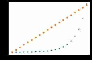
#  Check that each element is  True
# base  Of   Index is  linspace  What you get is  logspace
np.alltrue(2 ** np.linspace(0, 10, N)  == y2)
True️ Add : About array Condition judgment of
#  Can't be used directly  if  Judge  array  Whether a certain condition is met
arr = np.array([1, 2, 3])
cond1 = arr > 2
cond1
array([False, False, True])
if cond1:
    print(" This is not acceptable. ")
---------------------------------------------------------------------------

ValueError Traceback (most recent call last)

<ipython-input-184-6bd8dc445309> in <module>
----> 1 if cond1:
 2 print(" This is not acceptable. ")


ValueError: The truth value of an array with more than one element is ambiguous. Use a.any() or a.all()
#  Even if you're all  True  It doesn't work either
arr = np.array([1, 2, 3])
cond2 = arr > 0
cond2
array([ True, True, True])
if cond2:
    print(" Not yet ")
---------------------------------------------------------------------------

ValueError Traceback (most recent call last)

<ipython-input-187-7fedc8ba71a0> in <module>
----> 1 if cond2:
 2 print(" Not yet ")


ValueError: The truth value of an array with more than one element is ambiguous. Use a.any() or a.all()
#  We can only use any or all, This is easy to make mistakes , Please pay attention .
if cond1.any():
    print(" Just one for True Can , therefore —— I can ")
Just one for True Can , therefore —— I can
if cond2.all():
    print(" All values are True Can only be , I happen to be like this ")
All values are True Can only be , I happen to be like this
Create whole 1/0 array Shortcut to . It should be noted that np.zeros_like or np.ones_like, Both can quickly generate a given array equally shape Of 0 or 1 vector , It's in need of Mask Some locations may be used .
️ It should be noted that : created array The default is float type .
np.ones(3)
array([1., 1., 1.])
np.ones((2, 3))
array([[1., 1., 1.],
 [1., 1., 1.]])
np.zeros((2,3,4))
array([[[0., 0., 0., 0.],
 [0., 0., 0., 0.],
 [0., 0., 0., 0.]],

 [[0., 0., 0., 0.],
 [0., 0., 0., 0.],
 [0., 0., 0., 0.]]])
#  Like giving a directional amount  0  vector (ones_like  yes  1  vector )
np.zeros_like(np.ones((2,3,3)))
array([[[0., 0., 0.],
 [0., 0., 0.],
 [0., 0., 0.]],

 [[0., 0., 0.],
 [0., 0., 0.],
 [0., 0., 0.]]])
If you want to choose one of the most important in this section API, It must be random No doubt , Here we only introduce some commonly used 「 production 」 Data related API. They are often used to randomly generate training or test data , Neural network initialization, etc .
️ It should be noted that : Here we recommend the use of new API Way to create , That is, through np.random.default_rng() Mr Into Generator, Then on this basis, various distributed data are generated ( Memory is simpler and clearer ). But we will still introduce API usage , Because a lot of code is still old , You can mix a familiar look .
# 0-1  Continuous uniform distribution
np.random.rand(2, 3)
array([[0.42508994, 0.5842191 , 0.09248675],
 [0.656858 , 0.88171822, 0.81744539]])
#  Single number
np.random.rand()
0.29322641374172986
# 0-1  Continuous uniform distribution
np.random.random((3, 2))
array([[0.17586271, 0.5061715 ],
 [0.14594537, 0.34365713],
 [0.28714656, 0.40508807]])
#  Specifies the continuous uniform distribution of the upper and lower bounds
np.random.uniform(-1, 1, (2, 3))
array([[ 0.66638982, -0.65327069, -0.21787878],
 [-0.63552782, 0.51072282, -0.14968825]])
#  The difference between the above two is  shape  Different input methods , It's harmless
#  But in the  1.17  This is recommended after version ( In the future, we can use new methods )
# rng  It's a  Generator, It can be used to generate various distributions
rng = np.random.default_rng(42)
rng
Generator(PCG64) at 0x111B5C5E0
#  Recommended continuous uniform distribution usage
rng.random((2, 3))
array([[0.77395605, 0.43887844, 0.85859792],
 [0.69736803, 0.09417735, 0.97562235]])
#  You can specify upper and lower bounds , Therefore, this usage is more recommended
rng.uniform(0, 1, (2, 3))
array([[0.47673156, 0.59702442, 0.63523558],
 [0.68631534, 0.77560864, 0.05803685]])
#  Random integers ( Discrete uniform distribution ), No more than the given value (10)
np.random.randint(10, size=2)
array([6, 3])
#  Random integers ( Discrete uniform distribution ), Specify the upper and lower bounds and  shape
np.random.randint(0, 10, (2, 3))
array([[8, 6, 1],
 [3, 8, 1]])
#  The method recommended above , Specify the size and upper bound
rng.integers(10, size=2)
array([9, 7])
#  The method recommended above , Specify the upper and lower bounds
rng.integers(0, 10, (2, 3))
array([[5, 9, 1],
 [8, 5, 7]])
#  Standard normal distribution
np.random.randn(2, 4)
array([[-0.61241167, -0.55218849, -0.50470617, -1.35613877],
 [-1.34665975, -0.74064846, -2.5181665 , 0.66866357]])
#  The standard normal distribution recommended above
rng.standard_normal((2, 4))
array([[ 0.09130331, 1.06124845, -0.79376776, -0.7004211 ],
 [ 0.71545457, 1.24926923, -1.22117522, 1.23336317]])
#  Gaussian distribution
np.random.normal(0, 1, (3, 5))
array([[ 0.30037773, -0.17462372, 0.23898533, 1.23235421, 0.90514996],
 [ 0.90269753, -0.5679421 , 0.8769029 , 0.81726869, -0.59442623],
 [ 0.31453468, -0.18190156, -2.95932929, -0.07164822, -0.23622439]])
#  Gaussian distribution is recommended above
rng.normal(0, 1, (3, 5))
array([[ 2.20602146, -2.17590933, 0.80605092, -1.75363919, 0.08712213],
 [ 0.33164095, 0.33921626, 0.45251278, -0.03281331, -0.74066207],
 [-0.61835785, -0.56459129, 0.37724436, -0.81295739, 0.12044035]])
All in all , What I usually use is 2 Distribution : Uniform distribution and normal distribution ( gaussian ) Distribution . in addition ,size You can specify shape.
rng = np.random.default_rng(42)
#  Discrete uniform distribution
rng.integers(low=0, high=10, size=5)
array([0, 7, 6, 4, 4])
#  Continuous uniform distribution
rng.uniform(low=0, high=10, size=5)
array([6.97368029, 0.94177348, 9.75622352, 7.61139702, 7.86064305])
#  normal ( gaussian ) Distribution
rng.normal(loc=0.0, scale=1.0, size=(2, 3))
array([[-0.01680116, -0.85304393, 0.87939797],
 [ 0.77779194, 0.0660307 , 1.12724121]])
This section is mainly used to load the stored weight parameters or preprocessed data sets , Sometimes it's more convenient , For example, the trained model parameters are loaded into memory to provide reasoning services , Or time-consuming preprocessing data can be stored directly , Multiple experiments do not require reprocessing .
️ It should be noted that : There is no need to write the file name suffix when storing , It will automatically add .
#  Directly save the given matrix as  a.npy
np.save('./data/a', np.array([[1, 2, 3], [4, 5, 6]]))
#  Multiple matrices can exist together , be known as  `b.npz`
np.savez("./data/b", a=np.arange(12).reshape(3, 4), b=np.arange(12.).reshape(4, 3))
#  Same as the last one , It's just compressed
np.savez_compressed("./data/c", a=np.arange(12).reshape(3, 4), b=np.arange(12.).reshape(4, 3))
#  Load single  array
np.load("data/a.npy")
array([[1, 2, 3],
 [4, 5, 6]])
#  Load multiple , You can take out the corresponding... Like a dictionary  array
arr = np.load("data/b.npz")
arr["a"]
array([[ 0, 1, 2, 3],
 [ 4, 5, 6, 7],
 [ 8, 9, 10, 11]])
arr["b"]
array([[ 0., 1., 2.],
 [ 3., 4., 5.],
 [ 6., 7., 8.],
 [ 9., 10., 11.]])
#  The suffixes are the same , You just think it's no different from the one above
arr = np.load("data/c.npz")
arr["b"]
array([[ 0., 1., 2.],
 [ 3., 4., 5.],
 [ 6., 7., 8.],
 [ 9., 10., 11.]])
In this section, we array Start with the basic statistical attributes of , Yes, just created array Learn more about . It mainly includes the following aspects :
Are indicators related to descriptive statistics , For us to understand a array Very helpful . among , The most used are size related 「shape」, Maximum 、 minimum value , Average 、 Make a peace, etc .
The content of this section is very simple , You just need to pay special attention to ( remember ) Two important characteristics :
keepdims=True) in addition , For ease of operation , We use a randomly generated array As the object of operation ; meanwhile , We have designated seed, So every time , Everyone sees the same result . Generally, when we train the model , It is often necessary to specify seed, In order to 「 Same conditions 」 Adjust parameters under .
#   So let's create one  Generator
rng = np.random.default_rng(seed=42)
#   Regenerate into a uniform distribution
arr = rng.uniform(0, 1, (3, 4))
arr
array([[0.77395605, 0.43887844, 0.85859792, 0.69736803],
 [0.09417735, 0.97562235, 0.7611397 , 0.78606431],
 [0.12811363, 0.45038594, 0.37079802, 0.92676499]])
This section mainly includes : dimension 、 Shape and amount of data , And the shape shape We use the most .
️ It should be noted that :size No shape,ndim Indicates that there are several dimensions .
#  dimension ,array  It's two-dimensional ( Two dimensions )
arr.ndim
2
np.shape# shape , Return to one Tuple
arr.shape
(3, 4)
#  Data volume
arr.size
12
This section mainly includes : Maximum 、 minimum value 、 Median 、 Other quantiles , among 『 Maximum and minimum 』 We usually use the most .
️ It should be noted that : The quantile can be 0-1 Any fraction of ( Indicates the corresponding quantile ), And the quantile is not necessarily in the original array in .
arr
array([[0.77395605, 0.43887844, 0.85859792, 0.69736803],
 [0.09417735, 0.97562235, 0.7611397 , 0.78606431],
 [0.12811363, 0.45038594, 0.37079802, 0.92676499]])
#  The largest of all elements
arr.max()
0.9756223516367559
np.max/min# By dimension ( Column ) Maximum
arr.max(axis=0)
array([0.77395605, 0.97562235, 0.85859792, 0.92676499])
#  Empathy , Press the line
arr.max(axis=1)
array([0.85859792, 0.97562235, 0.92676499])
#  Whether to keep the original dimension
#  This needs special attention , Many deep learning models need to maintain the original dimension for subsequent calculation
# shape  yes  (3,1),array  Of  shape  yes  (3,4), Press the line , While maintaining the dimension of the row
arr.min(axis=1, keepdims=True)
array([[0.43887844],
 [0.09417735],
 [0.12811363]])
#  Maintain dimension :(1,4), original array yes (3,4)
arr.min(axis=0, keepdims=True)
array([[0.09417735, 0.43887844, 0.37079802, 0.69736803]])
#  One dimensional
arr.min(axis=0, keepdims=False)
array([0.09417735, 0.43887844, 0.37079802, 0.69736803])
#  Another use , But we are usually used to using the above usage , In fact, the two are the same thing
np.amax(arr, axis=0)
array([0.77395605, 0.97562235, 0.85859792, 0.92676499])
#  Same as  amax
np.amin(arr, axis=1)
array([0.43887844, 0.09417735, 0.12811363])
#  Median
#  Other uses and  max,min  It's the same
np.median(arr)
0.7292538655248584
#  quantile , Take by column 1/4 Count
np.quantile(arr, q=0.25, axis=0)
array([0.11114549, 0.44463219, 0.56596886, 0.74171617])
#  quantile , Take... By line  3/4, While maintaining the dimension
np.quantile(arr, q=0.75, axis=1, keepdims=True)
array([[0.79511652],
 [0.83345382],
 [0.5694807 ]])
#  quantile , Be careful , The quantile can be  0-1  Any number between ( Quantile )
#  If it is  1/2  Quantile , That's exactly the median
np.quantile(arr, q=1/2, axis=1)
array([0.73566204, 0.773602 , 0.41059198])
This section mainly includes : Average 、 Cumulative sum 、 variance 、 Further statistical indicators such as standard deviation . One of the most used is 「 Average 」.
arr
array([[0.77395605, 0.43887844, 0.85859792, 0.69736803],
 [0.09417735, 0.97562235, 0.7611397 , 0.78606431],
 [0.12811363, 0.45038594, 0.37079802, 0.92676499]])
np.average# Average
np.average(arr)
0.6051555606435642
#  Average by dimension ( Column )
np.average(arr, axis=0)
array([0.33208234, 0.62162891, 0.66351188, 0.80339911])
#  Another way to calculate the average  API
#  It is associated with  average  The main difference is ,np.average  You can specify weights , That is, it can be used to calculate the weighted average
#  It is generally recommended to use average, forget mean Well !
np.mean(arr, axis=0)
array([0.33208234, 0.62162891, 0.66351188, 0.80339911])
np.sum# Sum up , Not much said , similar
np.sum(arr, axis=1)
array([2.76880044, 2.61700371, 1.87606258])
np.sum(arr, axis=1, keepdims=True)
array([[2.76880044],
 [2.61700371],
 [1.87606258]])
#  Sum by column
np.cumsum(arr, axis=0)
array([[0.77395605, 0.43887844, 0.85859792, 0.69736803],
 [0.8681334 , 1.41450079, 1.61973762, 1.48343233],
 [0.99624703, 1.86488673, 1.99053565, 2.41019732]])
#  Sum by row
np.cumsum(arr, axis=1)
array([[0.77395605, 1.21283449, 2.07143241, 2.76880044],
 [0.09417735, 1.0697997 , 1.8309394 , 2.61700371],
 [0.12811363, 0.57849957, 0.94929759, 1.87606258]])
#  Standard deviation , Usage is similar.
np.std(arr)
0.28783096517727075
#  Calculate the standard deviation by column
np.std(arr, axis=0)
array([0.3127589 , 0.25035525, 0.21076935, 0.09444968])
#  variance
np.var(arr, axis=1)
array([0.02464271, 0.1114405 , 0.0839356 ])Literature and materials

One key, three links , Learning together ️